Chapter 30 Statistics and evidence-based practice
Introduction#
Many examinees approach medical statistics with a lot of apprehension. This is justified in most circumstances as we do not regularly practise statistics nor do we study it on a regular basis. Examiners are not different and appreciate this very well. You should remember that when you are asked questions related to medical statistics you are not expected to demonstrate the knowledge of asta tis tician. The examiners simply wish to satisfy themselves that as an inquisitive orthopaedic surgeon you understand the basic statistical concepts well enough to be able to scrutinize the published orthopaedic evidence. It is very unlikely that you will be asked esoteric questions (unless you do really well). Statistics of direct relevance (for example NJR survival analysis) are very popular with examiners and are frequently asked. Of the six basic science viva questions most of you would probably be asked at least one question related to
Medical Statistics.
What kind of statistics question you get asked in the viva would depend on the stage of your viva. If your Basic Science viva commences wit hastatis tics question this would be ase tiling ’ question designed to get you at ease. Remember when you answer your question to remain to the point, but whenever you can feel free to use buzzwords designed to show your familiarity and also to tempt the examiner onto your comfort zone.
Below are examples through which we aim to demonstrate what kind of questions you are likely to be asked and how to address them. The answers are deliberately but thoughtiully expanded to better understand the subject around that particular question and to help address potential f ollow-up questions.
Structured oral examination question 1#
What do these lines represent (Figure 30.1)?
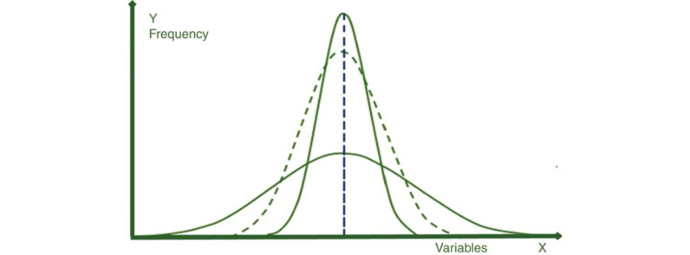
Figure 30.1 Bell-shaped curve normal distribution.
These are all bell-shaped curves of a ‘Normal’ distribution. The x-axis represents a variable (let it be weight, height, Hb level, Na level, hip score, knee score, etc.) and the y-axis represents the frequency of that variable.
Why do you say this is ‘Normal’?
A normal distribution of data is one in which the majority of data are relatively similar, occurring within a small range of values such as height, weight, Hb level, K, Na, etc. Ploting normally distributed data results in a bell-shaped graph as shown here (Figure 30.1).
What is the significance of this bell-shaped curve?
All normal distributions are symmetric and have bell-shaped curves with a single peak. They share important features that make statistical calculation and testing easy and reproducible. Two constant features of normally distributed curve are the mean, where the peak of the density occurs, and the standard deviation, which indicates the spread or girth of the bell curve. Although different variables yield different normal distributions, the y all satisfy the 68–95–99.7% rule. Sixty-eight of the observations f all within 1 SD of the mean, 95% of the observations f all within 2 SD of the mean and 99.7% of the observations f all within 3 SD of the mean. Moreover, in normally distributed data, the mean, median and mode are all the same value and coincide with the peak of the curve (Figure 30.2).
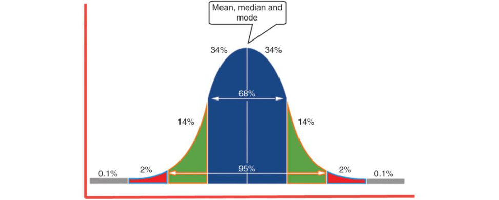
Figure 30.2 Normal distribution curve.
Why is it important to know whether your data are normally distributed or not?
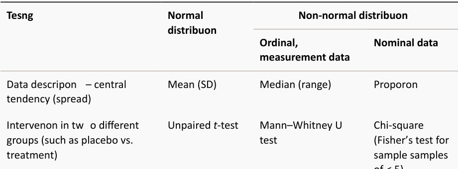
So that we can choose the best way to present, analyze and test our findings. For example, I would use mean and SD to present my normally distributed data in contrast to mode, median and range in non-normally distributed data. I would use parametric tests (such as t-test, analysis of variance (ANOVA)) in comparing my findings if data were normally distributed, but I would use non- parametric tests (such as Wilcoxon rank test, Mann–Whitney U tests) if I was dealing with non- normally distributed data.
Authors note 1: Describing data
Data are the building stones for any study and it is expected that all candidates are confident inunderstanding and describing data. In our experience most candidates are; however, there is some confusion about the pros and cons of various methods of presenting data. In this section, we summarize some important aspects.
Data in general are divided into:
1. Categorical data: the objects being studied are grouped into categories based on some qualitative trait; hence, they are also called qualitative data. This is furthered classified into:
a. Nominal: categories without order, e.g. smoking status, living status, marital status, etc.
b. Ordinal: categories with order, e.g. social status, ficat grading, and pain score (mild, moderate, severe), etc.
Either type can be binary (i.e. two categories only e.g. live or dead; married or unmarried;
smoker or non-smoker) or not binary.
2. Measurement data: the objects being studied are measured based on some quantitative trait. Hence, they are also called quantitative data. This is further classified into:
a. Discrete: only certain values are possible (there are gaps between the possible values), e.g. number of admissions to an orthopaedic ward, number of spinal metastases, number of patients transfused.
b. Continuous theoretically, any value within an interval is possible with a fine enough measuring device, e.g. age, height, weight, blood loss.
The type(s) of data collected in a study determine the type of presentation and statistical analysis used. Categorical data are commonly summarized using percentages or proportions and tested using Chi-square or Fisher exact tests. Summarizing measurement data depends on whether the data are normally distributed or not. If they are normally distributed they can be summarized using means and standard deviation and tested by parametric tests. If data are not normally distributed, they can be summarized using mode, median, range and tested by non-parametric tests (Table 30.1). It is not expected from candidates to know the details of these tests and when to use them. It is acceptable to use asta tis tic ians help to design a study. However, it boosts your answers if you have basic knowledge about the common ones (highlighted in the table).
There are several ways to check data for normality. Ploting normally distributed data produces a symmetrical bell-shaped curve. If the curve is not symmetrical, the data are probably not normally distributed Alternatively, data can be formally tested using the Kolmogorov–Smirnov testor Shapiro–Wilk’s test for normality. The latter tests are too sensitive to sample size and may show data as not normally distributed at the time the violation for normality is not substantive;
therefore, graphical methods are generally preferable.
Data can also be presented as risk ratio (RR) or relative risk. These are just ways of expressing chance in numbers. For example: 24 people skiing down a slope, 6 fall:
The risk = number of events of interest (falls) / total number of observations = 6/24 = 0.25
The odds = number of events of interest (falls) / number without the event (no falls) = 6/18 =
0.33
Relative risk or risk ratio (the y mean the same thing and are both abbreviated as RR) is simply the risk of the event in one group divided by the risk of the event in the other group. RR value of 1 means no difference between the two groups.
The risk difference (RD) is the risk difference between two groups. Sometimes this is called the absolute risk reduction and it is equal to risk on treatment – risk on control. RD value of 0 means no difference between the two groups.
The number needed to treat (NNT) is how many people would need to be treated for one extra patient to be helped and it is the inverse of RD.
The odds ratio (OR) is simply the odds of the e vent occurring in one group divided by the odds of the event occurring in the other group. OR value of 1 means no difference between the two groups.
There are pros and cons of using the above ratios. Odds ratios are hard to understand and are often misinterpreted. Risk difference (and derivatives like NNT) is more immediately useful than relative risk and odds ratio. The odds and risk ratio are equally variable whereas the risk difference varies more widely and less consistently. They do not change behaviour when the event of interest is reversed and work well in small samples and for rare events.
Table 30.1 Statistical tests.
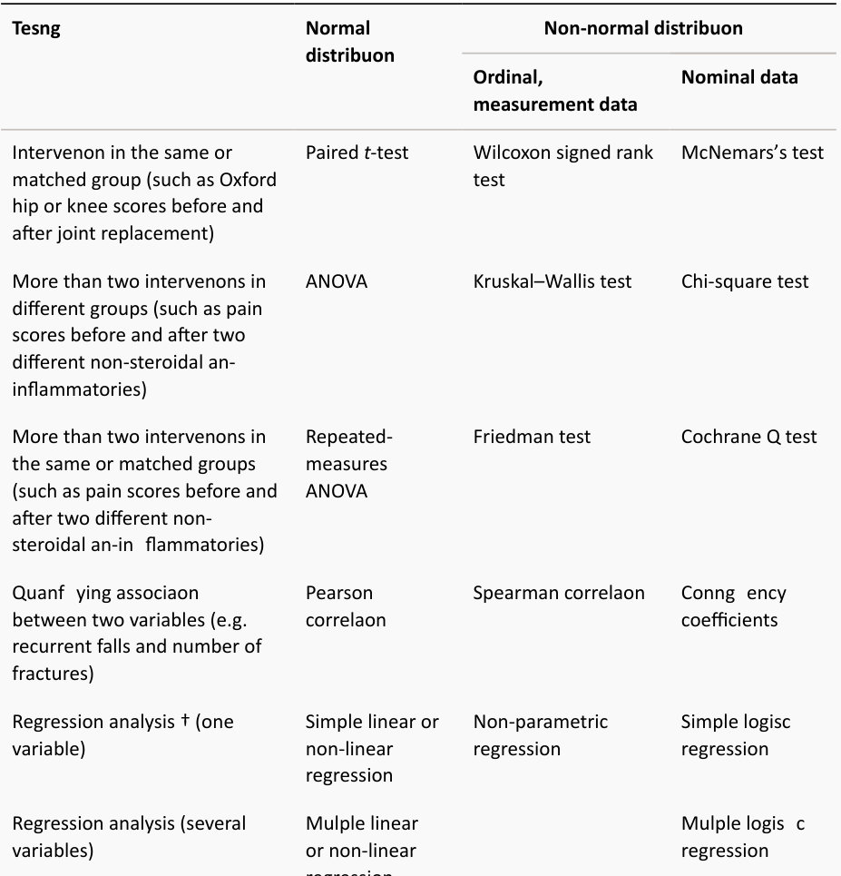
† Regression analysis involves modelling and analyzing several variables, when the focus is on the relationship between a dependent variable (for example, death) and one or more independent variables (for example, age, weight, comorbidities, haemoglobin le vel, etc.). It helps to understand how the dependent variable changes when any one of the independent variables is varied, while the other independent variables are held fixed.
OK, what about these two curves (Figure 30.3), are they also bell-shaped?
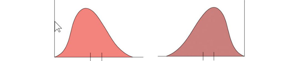
Figure 30.3 Skewed curves.
Not quite, they are skewed curves, they are not symmetric, and the tail is larger on the right for the first image and larger on the left for the second image respectively called right-skewed and left-skewed data.
What is the significance of skewed data and where is the mean in these images?
They are not symmetrical, therefore the mean is pulled by the outliers, so the mean lies toward the direction of skew (the longer tail) relative to the median. Hence the mean is larger than the median for right-skewed data and smaller than the median in left-skewed data.
What value would you use to describe this set of data?
I would use median and interquartile range.
OK, what is this chart (shown in Figure 30.4)?
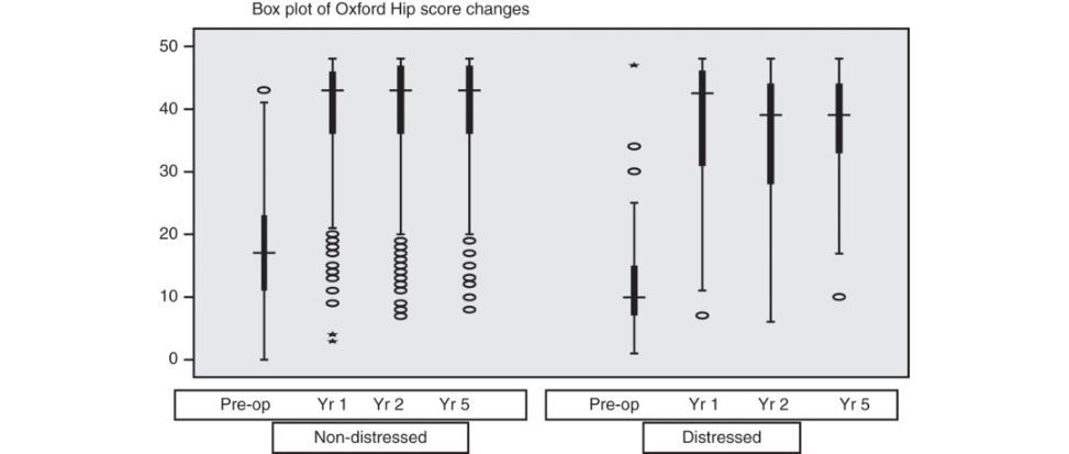
Figure 30.4 Box plot, Oxford hip score.
It is a box plot. It compares the Oxford hip score changes between distressed and non- distressed groups of patients from preoperative level to 5 years after surgery. This is another way to present findings graphically. It shows that in both groups of patients surgery resulted in improvement in Oxford hip score and also that there were more outliers in the non-distressed group compared to the distressed group, postoperative improvement was maintained at 5 years of follow- up and the distressed group appears to have made a comparable if not a slightly larger gain compared to the non-distressed group. This may be a better way to present skewed data graphically.
What are the different lines?
The width of the box shows the interquartile range, the line in the middle is the median value, the whisker shows the lowest and the highest values and the circles are the outliers.
What is an outlier?
A value that is much larger or smaller than the rest of the data.
Do you know how you can transform non-parametric data to more normal-looking data?
No.
OK, you can do logarithmic transformation or bootstrap technique, thanks.
Authors’ note 2
There are several ways to present data numerically and graphically. There is no perfect way and each one has pros and cons. Most candidates are familiar with bell-shaped curves, bar and pie charts. A box plot is another important and common way to present data and has been featured in the exam (Figure 30.5). The middle of the box plots represents the median and the sides (or theb oft om and top of the box) are always the first and third quartiles. The ends of the whiskers can represent several possible alternative values, such as the minimum and maximum of all of the data, one standard deviation above and below the mean of the data or the 9th percentile and the
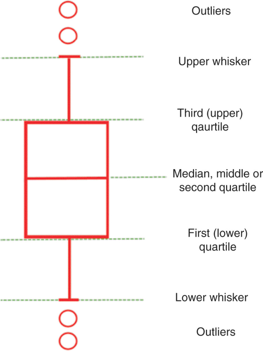
91st percentile. Outliers may be ploft ed as individual points.
Figure 30.5 Box plot.
Figure 30.6 compares the box plot to the bell-shaped curve for better understanding.
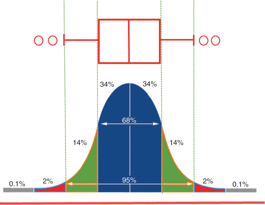
Figure 30.6 Box plot versus bell-shaped curve.
Structured oral examination question 2#
Can you tell me how you would design a clinical trial? Authors’ note 3 Frequently, candidates make the mistake of jumping straight onto a randomized controlled trial, the quest ionis designed to see if you have an overall concept of designing a trial and whether you might have any practical experience.
Design of a clinical trial would begin with a clinical question that might arise out of a clinical context. In the first instance I would conducta literature search utilizing the PIC O principle [a buzzword that would impress the examiner, PICO stands for Patients Intervention, Comparison, Outcome]. I would first search for the highest level of evidence in systematic reviews and meta- analyses. If there are none I would search for primary trials and so on [thus demonstrating that you are familiar with level of evidence]. If my search indicates that there is lack of evidence with regard to my clinical question I would proceed to designing a clinical trial. The design of the trial would depend on my underlying clinical question.
Tell me more about the level of evidence (Table 30.2). Table 30.2 Level of evidence.
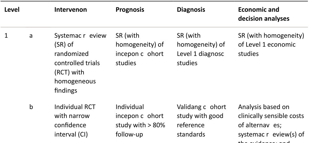
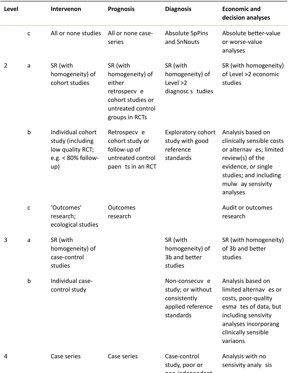
4 Case series Case series Case-control study, poor or non-independent reference standard
Level Intervention Prognosis Diagnosis Economic and decision analyses
5 Expert opinion Expert opinion Expert opinion Expert opinion
1. A complete assessment of the quality of individual studies requires critical appraisal of all aspects of the study design.
2. A combination of results from two or more prior studies.
3. Studies provided consistent results.
4. Study was started before the first patient enrolled.
5. Patients treated one way (e.g. with cemented hip arthroplasty) compared with patients treated another way (e.g. with cementless hip arthroplasty) at the same institution.
6. Study was started after the first patient enrolled.
7. Patients identified for the study on the basis of their outcome (e.g. failed total hip arthroplasty), called ‘cases’, are compared with those who did not have the outcome (e.g. had a successful total hip arthroplasty), called ‘controls’.
8. Patients treated one way with no comparison group of patients treated another way.
This chart was adapted from material published by the Centre for Evidence-Based Medicine, Oxford, UK.
For more information, please see www.cebm.net
Each published (or unpublished) study is considered as an evidence. The importance of this evidence is based on the quality of that particular study. The general principle of the hierarchy is that controlled studies are generally better than uncontrolled ones, prospective are generally better than retrospective and randomized are generally better than non-randomized studies [1]. Over the last three decades, several systems have emerged to assign a hierarchy for studies based on the aforementioned principles Examples of these systems are the Oxford Centre for Evidence-Based Medicine (OCEBM) [2], the Scotish Intercollegiate Guidelines Network (SIGN) [3] and the Journal of Bone and Joints Surgery Levels of Evidence [1]. I am familiar with the OCEBM, where the highest level of interventional studies is systematic reviews and meta-analysis of randomized controlled studies with a high homogeneity and the lowest is the expert opinion.
Authors’ note 4
Levels of evidence (LOE) are designed to help busy clinicians, researchers, or patients to find the likely best evidence in the shortest possible timeTable 30.1 showed the LOE produced by OCEBM.
These levels of hierarchy vary among different systems and over time. They are not absolute.
Sometimes ‘lower-level’ evidence from an observational study with a dramatic effect provides stronger evidence than a ‘higher-level’ study such as a systematic review of few studies leading to an inconclusive result. There are several examples in orthopaedic practice when a case series
(level IV evidence) changed practice significantly. Charnley hip replacement and Ponseti’s treatment of clubfoot are classical examples [4].
It is essential to appreciate that LOE are not recommendations for or against certain treatments and several factors must be considered when applying best evidence in practice. These include but are not limited to:
i. Is your patient sufficiently similar to the patient sin the studies you have examined?
ii. Does the treatment have a clinically relevant benefit that outweighs the harms (e.g.
medicine X reduces blood loss by 50 ml but may be clinically irrelevant)?
iii. Is another treatment better (e.g. a systematic review might suggest that surgery is the best treatment for back pain, but if exercise therapy is useful, this might be more acceptable to the patient than risking surgery as a first option) [ 5]?
Suppose that you are trying to test a new treatment? Literature search revealed no useful information.
Ideally, I would like to design a randomized controlled trial (RCT) to compare my new treatment to the current (or any another treatment). It is the most rigorous way of determining whether a cause–effect relation exists between treatment and outcome. Good RCT design must ensure [6]: 1. Random allocation to treatment groups. 2. Patients and trialists remain unaware of which treatment was given until the study is completed: this is called ‘concealment’. 3. The number of participant sis optimum to show a clinically relevant difference. 4. The two groups of treatment are treated identically except for the experimental treatment. The analysis is focused on estimating the size of the difference in predefined outcomes between intervention groups. There are two types of RCT; explanatory and pragmatic. It can be debated which one is better in this scenario.
What is the difference between the two types?
Explanatory trials generally measure efficacy – the outcomes of treatments under ideal conditions. F or example, if I was testing a new type of cement to help reduce revision rates, I would design my study in such a way that I remove or minimize the effect of any factors that could influence the revision rate. For example, all operations will be done by surgeon X, incentre X using implant X, at room temperature X and using a standardized cementing technique, etc. This design would belikely to show me the real effect of the new cement on revision rate. However, inreality the above design is neither practical nor desirable because we would want to see the tested intervention (the new cement here) work similarly in every centre, for every surgeon and with every implant. Hence the pragmatic trials are more popular. They measure effectiveness – the benefit the treatment produces in routine practice [ 7].
How do you randomize?
There are manyways of randomization. Ideally this should be performed by a centralized computerized system.
What is the advantage of randomization?
The advantage of randomization ist o avoid bias by equally distributing the known and unknown patient variables (that potentially affect the outcomes) so that the difference in treatment effect is most likely to be due to the difference in the intervention.
What do you mean by bias?
Bias is a tendency to deviate from the true value due to an error in the study design and thus over- or underestimate the true value of the treatment effect. Examples of bias include selection bias allocation bias, assessment bias, performance bias, etc.
Once you complete your trial how would you know if the new treatment is effective or not?
I would perform asta tis tical test and if the P value is < 0.05 this would suggest that there isless than 5% chance that the observed difference in treatment effect is purely due to chance, therefore I would consider the result to best atis tic ally significant.
Would you change your practice based on the results of a P value? Can you imagine a situation where the P value is > 0.05 but you might want to reconsider the intervention?
Yes, where there is a possibility of a type II error.
What is a type II error?
Where the sample size of the trial might be inadequate and therefore even if there was a significant difference between the intervention and the control group this would not be evident in the statistical test.
OK, this is known as the power of the study. Time’s up. Thankyou.
Authors’ note 5
Questions about designing RCT are very popular in the FRCS exam. Good understanding increases your marks, even if you do not have personal experience inrunning a trial. This section summarizes the essential concepts and buzzwords that you need to deliver when you are asked about RCT.
Research is conducted to answer a particular question. Although RCT is the most rigorous way of determining whether a cause–effect relation exists between treatment and outcome, it is not the only way. RCT is conducted to an ethically approved protocol that prospectively sets out its rationale conduct and plan of analysis. Important design considerations include the following.
1. A literature search to establish current knowledge, thus refining the research question and trial methods to take knowledge forward and avoid unnecessary research repetion. T rials are often very expensive and sometimes adequate answers can be found either from the literature or alternative study designs. Information from a previous published work is important to calculate the required sample size.
2. Sample selection and generaliz ability: participants should be representative of the population of interest. Thus, inclusion and exclusion criteria are important trial design features and should be carefully thought about, e.g. excluding pregnant women for safety reasons is often a valid reason for exclusion. However, excluding patients with dementia because consenting is more problematic is not a good reason and may not be ethically acceptable. This would deprive such patients from future evidence-based treatment.
3. Primary and secondary outcomes: the primary outcome (or the primary endpoint)
represents the greatest treatment benefit. Some trials have more than one primary outcome if several outcome measures are of equal importance. Secondary outcomes (or secondary endpoints) may provide information on therapeutic effects of secondary importance, side effects, or tolerability. Both should be clinically relevant, valid, reproducible and sensitive to detect changes. For example, set inga trial to investigate the value of tranexamic acid in reducing blood loss in joint replacement. Blood transfusion is a good primary outcome. It can be measured easily, accurately and has importance topa tien t and surgeons. In comparison, drain blood loss, although important, does not tick all the boxes mentioned earlier , hence it is better used as a secondary outcome rather than a primary one (see also the type of data section).
5. Sample size (power). A well-designed study should have the optimal number of participants adequate sample size) to provide an adequate chance of finding a clinically worthwhile difference between treatments. Over-recruitment is undesirable as it is uneconomic and unethical (exposing more patients to an ‘unnecessary’ experiment when the answer has been established within reasonable bounds). A smaller number of participants may cause a type II error (not finding a difference between the two treatments although there is a difference).
Sample size is usually calculated for the primary outcome and the following elements are required for calculation:
Chosen significance level (usually 5%).
Study power (typically 80% or 90%).
Chosen clinically important difference in the primary outcome.
The variability in response (standard deviation in the primary outcome).
There are several pieces of sotiw are or websites that provide this calculation.
6. Bias: refers to systematic err or in trial design, conduct, analysis or reporting. The true effect of the treatment under investigation is systematically under- or overestimated For example:
i. Question bias : e.g. comparing a new treatment with the most poorly performing alternative will inflate the apparent benefit of the new treatment.
ii. Sampling bias: patients with significant comorbidity are excluded from trial or decline to participate limiting the g eneralizability of findings.
iii. Selection bias : patients with underlying prognosis are systematically assigned in larger numbers to one treatment than another.
iv. Information bias : including any of a range of factors that distort the recording of data, e.g. measurement error, recall bias, workup bias, interviewer bias, misconduct.
v. Windowing bias: where the investigators’ prejudices influence the selection and presentation of findings.
vi. Publication bias : studies with negative or no difference are less likely to be submift ed, published, quoted or even read.
7. Randomization : if adequately conducted, randomization reduces the chance of selection bias because known and unknown prognostic influences are distributed by chance among the different treatment groups.
8. Blinding (masking or concealment): if researchers or patients have a preference for a particular treatment, this can introduce bias. Blinding is an important design feature to manage both explicit and implicit prejudice, although it is not always possible.
9. Analysis: this is conducted according to a protocol agreed prospectively before any analysis has begun. Three approaches are described:
i. Intention-t o-treat (ITT), meaning that participants are analyzed according to the group allocated regardless of whether they continued with that treatment. IT Tis widely considered as the golden standard to analyze RCT because it avoids the bias associated with the non-random loss of the participants.
ii. As-treated analysis: comparing the groups according to the treatment that they received. It does not consider which treatment they were allocated to.
iii. Per protocol analysis includes participants who metall the protocol criteria in the terms of the eligibility, interventions, out come assessment and followup.
The cons of the last two analyses are that they potentially overestimate the efficacy of an intervention resulting from the removal of non-compliance and protocol deviations which are likely to occur in actual clinical practice.
10. Logistics (ethics approval, local approval, building and training a research team).
Structured oral examination question 3#
If you had the choice of deciding between a highly sensitive testor a highly specific test to diagnose as many of the diseases as possible for a particularly debilitating condition, what kind oftest would you go for?
I would choose a highly sensitive test.
Why is that?
In a highly sensitive test more of the diseased cases would be positive whereas a highly specific test might miss some disease cases.
What are the drawbacks of each?
A highly sensitive test may pickup more false positive cases and create unnecessary patient anxiety, whereas a highly specific test might have more false negative cases and miss some diseased cases.
What if you wanted to confirm diagnosis of the disease?
I would choose a highly specific test.
Do you think hip ultrasound is a good screening test for DDH?
Yes, ultrasound ticks most of the WHO criteria for a screening testitis accepted and tolerated by patients and parents, it is safe, it has a high sensitivity to detect the disease before a critical point and has high specificity to reduce false positives.
Should we screen all newborns for DDH using ultrasound?
This is widely debated. Some countries have already started a universal screening programme and showed encouraging results; others opted for a selective screening programme to reach an acceptable cost–effectiv eness ratio. To run a successful screening programme,several criteria should be met. These criteria can be categorized into three groups: 1. Disease criteria. i. Disease with significant impact on community. ii. Natural history of the disease is known. iii. Detection occurs before a critical point (before it is too late). 2. Screening test features. i. Accepted and tolerated by patients.
ii. High sensitivity to detect the disease before the critical point.
iii. High specificity to reduce false positives.
iv. Cost-effectiv e.
3. Screened population features.
i. Disease has high enough prevalence to allow screening.
ii. Accepted and effective treatment is available.
iii. Patients are willing to undergo further evaluation and treatment.
DD Has a disease fulfils most (and not all) of these criteria. The condition is ‘important’ with an accepted treatment and suitable facilities available for that treatment. There is an early stage in which DDH can be picked up, with a sensitive test that is acceptable to the population. However, there is no universal agreement on who should receive treatment and who should not. Furthermore, the cost of the screening programme in comparison to the full costs of delayed detection (including medicolegal costs) has not been established [8].
Authors’ note 6: Diagnostic tests
Sensitivity , specificity, positive and negative predictive values of a diagnostic test are commonly featured in the exam. Most candidates are aware of this, yet find it difficult to recall and present their answers succinctly to achieve a high mark to reflect their knowledge. Our advice is to understand the definition rather than memorizing it.
1. Sensitivity (Sn): the probability of identifying a disease (true positive when the disease is present (true positive + false negative).
Sn = true positive / true positive + false negative.
2. Specificity (Sp): the probability of excluding a disease (true negative when the disease is not there (true negative + false positive).
Sp = true negative / (true negative + false positive).
3. Accuracy (A): the probability of correct identification of a disease.
A = true positive + true negative / total number.
4. Positive predictive value (PPV): the probability of someone having a disease (true positive)
when they have tested positive all the positives = true positive + false positive).
PPV = true positives / (true positives + false positives).
5. Negative predictive value (NPV): the probability of someone not having a disease (true negative when they have tested negative all the negatives = true negative + false negatives).
NPV = true negatives / (true negatives + false negatives).
Unlike sensitivity and specificity , predictive values are properties of the t est interacting with the prevalence of disease in the population. A high PP V indicates a strong chance that a person with a positive test has the disease in populations with high prevalence of the condition being examined (true positive is high in such population whereas a low PP Vis usually found in populations with low prevalence of the condition being examined.
6. Likelihood ratio (LR): the ratio of the chances of truly having a disease to not having it, given that a positive test result was obtained.
LR = Sn / (1 – Sp).
We can calculate the LR for every test. The larger the LR, the better the test. Increasing sensitivity and/ or specificity would increase the LR (a better test) and vice versa (you can check this by replacing random numbers in the formula).
Ploting Sn against (1 – Sp) produces a characteristic curve called ‘receiver operating characteristic ’ (ROC) curves (see Figures 30.7 and 30.8). An ideal ROC curve rises quickly to the upper left corner of the graph (high Sn and Sp) and stays high, leaving a larger area under the curve. A poor ROC curve rises slowly and has less area under the curve. The overall shape of a testis determined by physical law, biochemical properties, or the financial resources used in the design or manufacturing of the test. Once the overall ROC curve is fixed, the surgeon or experimenter decides how to use the test by choosing a cut-off value. Different cut-off values result in a balanced testor a test that is optimized for use in screening or confirmation (Figure
30.9).
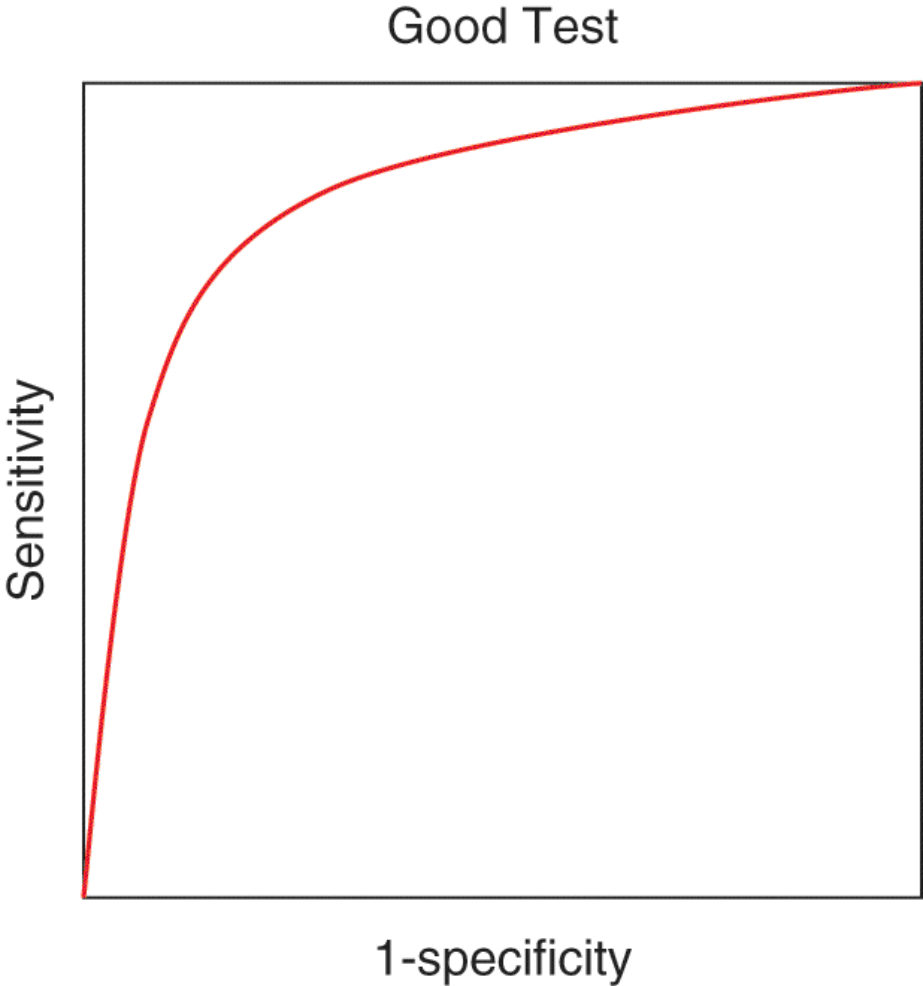
Figure 30.7 Good ROC curve.
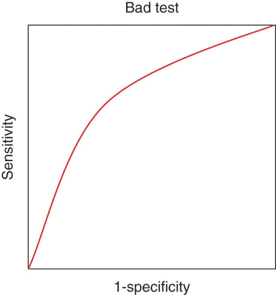
Figure 30.8 Bad ROC curve.
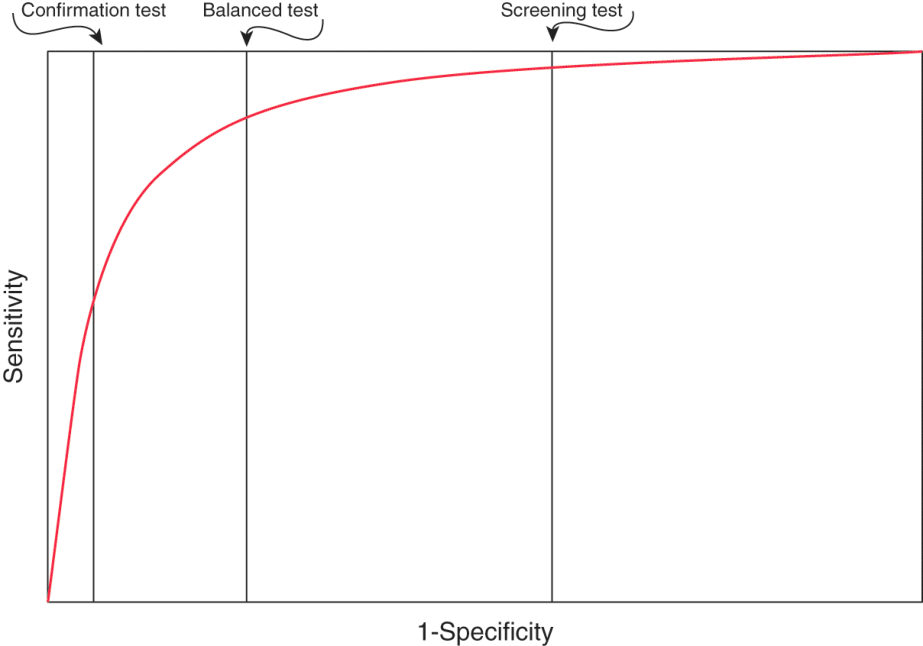
Figure 30.9 Different cut-off values result in a balanced testor a test that is optimized for use in screening or confirmation.
Structured oral examination question 4#
This is an abstract of an RCT comparing TXA to placebo to reduce blood transfusion in total knee replacement (Figure 30.10). Please, read the result section and t ell me your thoughts of the findings.
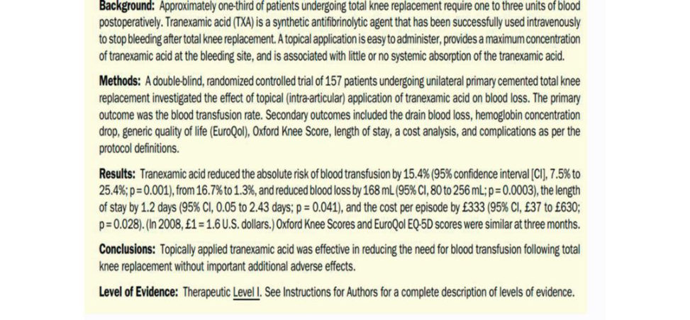
Figure 30.10 Journal abstract.
The results of the trial showed that TX Ahas been effective in reducing blood transfusion rates by 15.4% (from 16.7% to 1.3%). That was statistically significant (P = 0.0001). The trial also showed that TXA statistically significantly reduced blood loss. As a surgeon, I consider the first findings are clinically important, but I cannot say the same about the amount of blood loss. Although it is statistically significant, it is not clinically. The same could be said about the length of stay and cost.
What do you think about the 95% confidence interval?
The 95% CI for the blood transfusion was 7.5–25.4%; a reasonably narrow CIA confidence interval shows the range within which the treatment effect is likely to lie if the study was repeated again. In other words, if this trial was repeated 100 times, then 95 out of those 100 times, the absolute reduction of blood transfusion would lie within between 7.5% and 25.4%.
How is CIre lated to the P-value?
A P-value is calculated to assess whether a treatment effect observed in a study is likely to have occurred simply through chance. Traditionally , researchers accept a P-value of less than 0.05. This means that there is a 5% risk that the result I have seen in my study happened by chance and 95% is a true effect of the intervention that I am testing. So , in the above study, there is 1 in 1000 (P = 0.001) risk that the 15.4% reduction in the transfusion rate happened by chance and not because of the TXA. For the same reason we should be careful not to discount studies when the P-value is close but higher than 0.05. In comparison to CI, the P-value does not give any idea about the treatment effect.
Which one would you prefer?
CIs are preferable to P-values, as they tellus the range of possible effect sizes. CIs aid interpretation of clinical trial data by puting upper and lo wer bounds on the likely size of any true effect. A CIt hat includes no difference between treatments indicates that the treatment under investigation is not significantly different from the control.
You mentioned that the CI of the above study was narrow. Would you prefer a narrow or a wide CI?
I would prefer a narrow CIas this indicates we are more certain about the possible range of treatment effects. A wide CI indicates that we are more uncertain about the range. A suitable example might be of a confident candidate who is 95% confident to have scored between 70% and 80% in his FRCS exam. Contrast this with another candidate who is equally (95%) confident to have scored between 40% and 90%. In other words, the P-value gives you statistical significance, but CIg ives you clinical significance.
Could the above study findings be wrong and TXA does not reduce blood transfusion?
Yes, this is called type I error when a study concludes that a supposed effector relationship exists when in fact it does not. Another example is when a test shows apa tien t to have a disease when in fact the patient does not have the disease.
How does it differ from type II error?
If this study failed to show that the TXA reduces blood transfusion when really it does, this is type II (Figure 30.11).
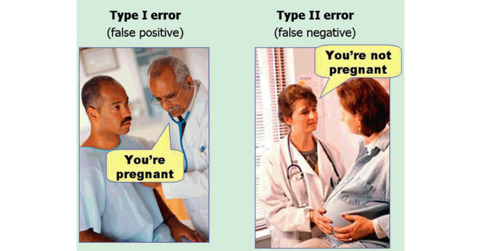
Figure 30.11 Type I and II errors.
Which one is worse?
Both should be considered and minimized. The seriousness of the implication may vary depending on the scenario. A new test that fails to detect a cancer when it is there (type II error) is serious. Another test that shows cancer when it is not there (type I error) and the patient then undergoes unnecessary surgery is serious too.
How do you minimize errors?
An integral part of a research study is to formulate and test a hypothesis. Because the testis based on probabilities, the reis always a chance of making an incorrect conclusion (type I and type II). Inst atis tical terms, type I error occurs when the null hypothesis is true and gets rejected. The probability of making a type I error is related to the level of significance (P-value or α) we set for our hypothesis test. A P-value of 0.05 indicates that we are willing to accept a 5% chance that we are wrong when we reject the null hypothesis. To lower this risk, we can lower the P-value. The drawback is that we will be less likely to detect a true difference if one really exists. The probability of making a type II error is related to the size of the study and the power of the test to detect a difference in the primary outcome. We can minimize type II error by increasing the size of the study and/or ensuring our test has enough power (for example, using Hb level drop rather than swab weights to measure blood loss).
What is the null hypothesis?
As I mentioned earlier , an integral part of a research study is to formulate and test hypotheses. The null hypothesis is normally the default position, eg. that there is no difference between a new and an old treatment. The null hypothesis is paired with a second alternative hypothesis, e.g. there is a difference between treatments. This is because it is easier to prove something exists rather than does not exist. For example, I cannot reject the statement ‘all cats are white’ by showing you 1000 white cats. However, I could reject it by showing you one black cat!
Structured oral examination question 5#
Have a look at Figure 30.12. Do you know what this plot is?
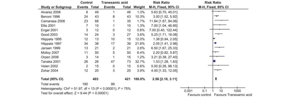
Figure 30.12 Forest plot.
This is called a forest plot (also known as a blobbogram). It numerically and graphically represents a meta-analysis which combines results from a number of studies addressing the same question.
What is the difference between a review and meta-analysis?
A clinical review simply locates and summarizes the findings of several studies. However, a systematic review is a rigorous and prestructured approach to conducting are view. The researchers decide beforehand on their inclusion and exclusion criteria, how they will search the literature, extract data, synthesize and analyze them. The meta-analysis is another stage in conducting systematic reviews when authors combine data from different studies statistically with a view to get inga combined and more precise estimate of the interventions effectiveness This is not always possible due to data limitations.
Why do we need reviews and meta-analyses?
For many surgical procedures, there have been a number of clinical studies and it would seem natural to want to combine them to get the most comprehensive overview of the effect of treatment. Properly conducted systematic review and meta-analyses with homogeneity are considered the highest level of evidence in clinical practice.
What do you mean by homogeneity?
In a meta-analysis, investigators combine results from reasonably similar studies. However, findings from these studies are likely to vary due to different methodologies (randomized or not, how allocation is concealed, blinding, etc.); patients inclusion and exclusion criteria); interventions (type, dose, duration, etc.); outcomes (type, scale, duration of followup and usage). Such variations can introduce heterogeneity into study findings (variation greater than that expected by chance).
Heterogeneity can be formally tested using the χ2 heterogeneity testor Q statistic The significantly high Q test suggests heterogeneity. Homogeneity conversely means that the variations among the study are low and the results of each individual study are compatible with a single underlying treatment effect.
Cochrane sotiw are (RevMan) produces I2, which is the proportion of variation that is due to heterogeneity rather than chance. Roughly, I2 values of < 50% indicate low, 50–75% indicate moderate, > 75% indicate high heterogeneity.
Back to Figure 30.12; can you explain the findings?
The forest plot represents 14 studies comparing tranexamic acid (TXA) to the control. It is not clear whether the control is a placebo or another medicine. This may be clarified in the methodology section. The forest plot consists of several columns: 1. The first column lists the names of the studies and the date of publication. These can be ordered alphabetically (as in this example) or by the year of publication, the weight of the studies or the treatment effects. 2. The second column represents the events in the TXA group. Again, it is not clear which event the plot represents. It could be blood transfusion, DVT or PE rates. (Examiner: it is blood transfusion rates.) 3. The third column represents the number of participant sin the TXA group. 4. The fourth column represents the events in the control group. 5. The fitih column represents the number of participant sin the control group. 6. The sixth column is the weight that is given to each study. The weight reflects the precision of the study (size and CI). Tanaka 2001 is the highest weighted study (32.7%). 7. The seventh column represents the treatment effect estimate. In this example it is the risk ratio which is equal to (events/total of the control) divided by (events/total in the TXA group). The risk ratio is one of several ways of presenting proportions: others are odds ratios and risk differences. 8. The last column provides a plot of the measure of effect for each study. The area of each square is proportional to the study’s weight in the meta-analysis. The higher the weight of the study the larger the square (see Tanaka 2001). On each side of the square there is a horizontal line representing the confidence interval. The narrower the CI the more precise the study is. The plots of the weighted effects are scattered on each side of aver tical line representing the no effect line. Here, the no effect line passes through 1 because it represents a risk ratio. It would be 0 if it was a risk difference.
Depending on the outcome of each included study, it can lie on either the left or the right side of the no-effect line. In this example, they all lie to the right of the no-effect line. The further away from the line, the more profound the effect. The overall effect is represented by a diamond. If a study plot touches the no-effect line, it means that its effect does not differ from no-effect for that individual study. The same applies for the diamond (the overall measure of effect): if the points of the diamond overlap the line of no effect the overall result is ‘no effect’ at the given level of confidence. In this study, the diamond position favours TXA.
That is very good. What about the word ‘fixed’ and the letters ‘M-H’? What do they signify?
The Mantel–Haenszel (M-H) testis used to combine studies in this plot; this is used by the Review Manager (RevMan 5) sotiw are that was developed by Cochrane library. The word ‘fixed’ refers to the fixed-effects model. One of two models used in meta-analysis. The other is called the random-effects model. In the fixed-effects model, it is assumed that the size of the effect is similar in the included studies. In this example, the size of the effect is a participant who had a blood transfusion. It is reasonable to assume the size of the effect is similar and use the fixed-effects model.
Can you give me an example where a random-effect model should be used?
Yes, when the effects are not similar. For example, combining data from two different outcome measures such as Oxford hip score and Harris hip score. Although they measure the hip function, the y are not the same.
How would you interpret the finding in the plot?
The plot shows that TXA reduced the risk of transfusion by 2.56 times with 95% CI (2.10 – 3.11) and P-value 0.00001 (the test for overall effect). This is statistically and clinically significant. However, there is significant heterogeneity as evident by the high I2 value (75%) and this was statistically significant (P-value < 0.00001). So, my interpretation for the above finding is that there is evidence that TXA does reduce the blood transfusion, but it is difficult to quantify (soth eRR of 2.56 shows it is not necessarily true).
How to deal with heterogeneity?
I expect the authors to explore this heterogeneity further. There are several options to do so: 1. One option is that of not performing a meta-analysis in the first place. They can simply present the findings as a table without pooling them. 2. Subgroups analysis of studies that are more similar. For example, studies with a high dose of TX Aor those receiving TXA earlier rather than later, etc. to see whether this could explain the heterogeneity. 3. In this example, the authors used the fixed-effects model for combining studies. Using the random-effects model may uncover some of the heterogeneity.
4. Investigating heterogeneity using meta-regression. Meta-regression is an extension to subgroup analyses that allows the effects of multiple factors to be investigated simultaneously. It is similar to simple regressions, in which an outcome variable is predicted according to the values of one or more independent variables. In the above example, the outcome variable is the effect estimate (RR). The independent variables are characteristics of studies that might influence th eRR such as dose, timing of administration, the use of heparin, the use of transfusion protocol, etc.
Figure 30.13 is another plot of meta-analysis. In fact, it is from the same meta-analysis in Figure 30.12. Do you know the name of this plot?
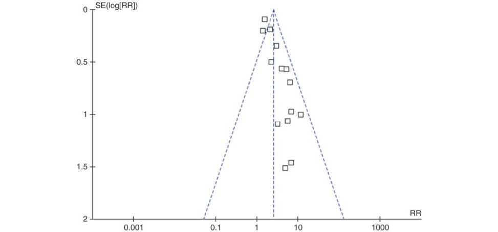
Figure 30.13 Funnel plot.
This is called a funnel plot which is a simple scatterplot of the treatment effects (risk ratio – horizontal axis) from individual studies (small squares) against the precision of the studies represented by standard error (SEver tical axis). SE is the standard deviation divided by the square root of the sample size. Hence, the larger the study, the lower the SE. It is expected that larger studies (big sample size) are more precise (low standard errors) and will be scattered very close to each other around the pooled effect at the top of the plot. The smaller studies are scattered widely toward theb oft om, giving the classical inverted symmetrical funnel. The funnel plot shows trials scattered asymmetrically around the pooled RR with small trials having greater effect. There are two explanations for these findings. This may be due to smaller trials of lower quality tending to overestimate the true effect; hence they are on the right side of the pooled effect. It might also reflect publication bias, where small trials that did not show benefit were not published (publication bias).
Authors’ note 7
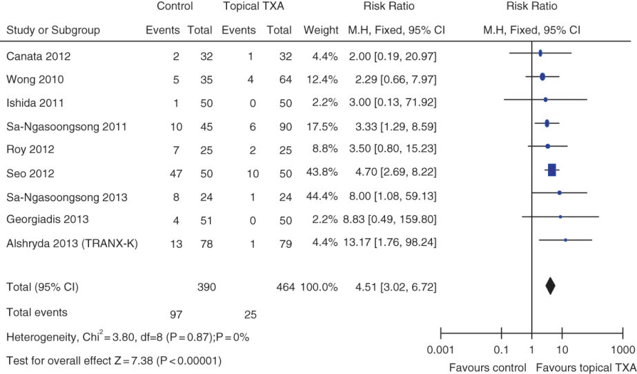
See the below figures for comprehension: Figure 30.14 showed that I2 is 0% and there is no significant heterogeneity in the included studies. So, the conclusion is that topical TXA reduced blood transfusion significantly by 4.5-fold. The same studies were displayed in a funnel plot
(effects against SE) and the plot showed the studies distributed symmetrically around the effect line (4.5 RR), indicating that publication bias is not likely (Figure 30.15).
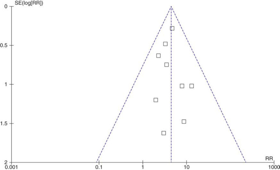
Figure 30.14 Forest plot with homogeneity.
Figure 30.15 Funnel plot with symmetrical distributions of the studies around the effect line.
Structured oral examination question 6#
The following plot (Figure 30.16) is from the Norwegian Joint Registry about the effect of cement on the implant longevity. Can you describe the findings?
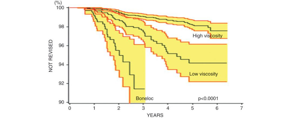
Figure 30.16 Survival analysis curve.
This is a survival analysis of Charnley femoral prostheses using different types of cements (high-viscosity, low-viscosity and Boneloc). There is asta tis tic ally significant difference between the three groups (no overlaps in the confidence interval and P-value < 0.0001). The high viscosity cement seems to provide a higher survival rate where about 98% survived to 6 years.
What is a survival graph, why do you need this, could you not simply measure mean survival with CI?
Well, a survival graph measures ‘timet o event’, this graph looks at survival probability and every time the e vent takes place survival is recalculated.
What are the different lines in this chart?
The midline is the mean value and the upper and lower lines represent the CI.
Why did the upper and lower lines diverge towards the right?
This is because as the study progressed there were fewer patients remaining in the study. With a lower number of patients the precision of the study and the confidence about the findings become low; therefore, the CI becomes wider.
Looking at this chart, can you predict the survival probability at 20 years?
No, it is not possible to estimate survival probability beyond the maximum follow-up period of the study.
Can you estimate the mean revision time?
No, we cannot as there are differing follow-up times, we can only estimate the cumulative risk of revision.
What do you understand by ‘censored data’?
If apa tien t diesis lost to follow-up or withdraws from the study then data from that patient are incomplete or censored.
So, are censored data wasted then?
No, they contribute data until the point of censoring.
Have you noticed an y, can you tell me if there is a problem with this chart?
Yes, the CI for Boneloc and low-viscosity cement is very wide, and I suspect the population at risk was low, but the numbers are not indicated.
The below plot is from the National Joint Registry of England and Wales (Figure 30.17). Take a look at this chart and tell me what you understand.
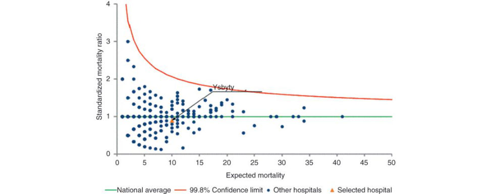
Figure 30.17 National Joint Registry report.
This shows the 90-day mortality rate following joint replacement (not specified in this chart whether hip or knee replacement) for a selected hospital (orange triangle). Similar charts are produced for individual surgeons (not shown in this figure). Here the y-axis denotes standardized mortality ratio which is the proportion of deaths compared to the average, the x-axis denotes the expected adjusted mortality for the involved hospitals. The data are ‘risk-adjusted’ to take account of the fact that different hospitals may operate on higher-risk or lower-risk patients (e.g. because of demographics in the patient population the y work with). Although case-mix adjustment is a useful tool, as with any methodological approach it cannot account for all differences including those that may be due to random events. The central green line denotes the average national expected mortality and the redline denotes the 99.8% confidence limit. Progression along the x-axis means that the hospital has done more cases and/or cases at a higher mortality risk, such as older patients Progression along the y-axis means the hospital has had more deaths. The y-axis figures are presented as a ratio. This means the values do not represent percentages of patients who have died, but they represent the proportion of deaths compared to the average.
Hospitals on the green (horizontal) line have the average expected mortality taking into account their case mix and number of cases. Hospitals on either side of the green line but below the upper redline have had a level of mortality (when taking into account their case mix and number of cases)
that is within the expected range. Hospitals above the top redline (which represents a ‘99.8%
Confidence Limit line’) would have a mortality rate that is higher than expected.
So, how did this hospital do?
The hospital’s mortality was well within the expected mortality range.
Can you tell me anything about the type of patients the hospital operated on?
Yes, we can see that the orange triangle is not far along the x-axis denoting that the hospital did not perform surgery on patients with higher expected mortality.
Authors’ note 8: Survival analysis
Survival analysis originally studied time from treatment until death, hence the name, but survival analysis is applicable to many other areas as well as mortality. It estimates the time between entry to a study and a subsequent event. Events may include death, injury, revision of an implant, recovery from illness (binary variables) or transition above or below the clinical threshold of a meaningful continuous variable (e.g. CD4 counts in HIV infection). It also compares time-t o-event between two or more groups, such as cemented vs. non cemented in total hip replacement.
Moreover, it assesses the relationship of co-variables to time-t o-event, such as antibiotic in cement, hinged design, weight of the patients, LMWH, etc.
The following are important definitions.
the time from entry into a study until a subject has a particular outcome. This is
Time-to-event: represented by a drop on the survival curve.
subjects are said to be censored if they are: (1) lost to follow-up or (2) dropout of
Censoring: the study, or (3) if the study ends before they die or have an outcome of interest.
Censored subjects are represented by a tick mark on the survival curves (Figure 30.18).
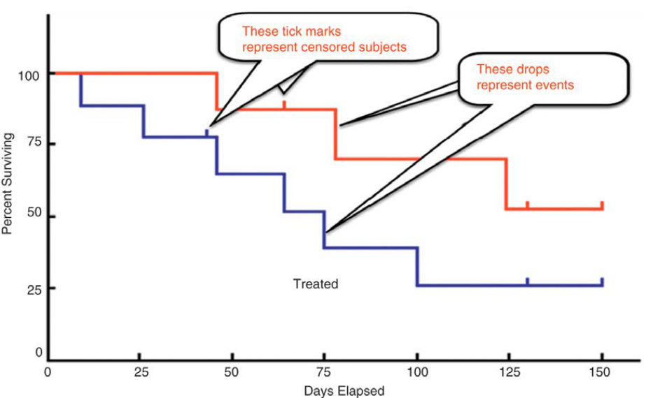
Figure 30.18 Survival curves.
The Kaplan–Meier survival curve is a non-parametric estimate of the survival function. Simply put, it is the probability of surviving past certain times in the sample (taking into account censoring). Three assumptions are made in survival analysis:
1. We assume that at any time patients who are censored have the same survival prospects as those who continue to be followed.
2. The survival probabilities are the same for subjects recruited early and late in the study.
3. We assume that the event happens at the time specified.
The Kaplan–Meier computes the probabilities of occurrence of the event at a certain point of time by multiplying these successive probabilities by any earlier computed probabilities to get the final estimate For each time interval, survival probability is calculated as the number of patients surviving divided by the number of patient sat risk. Patients who have died, dropped out, or move out are not counted as ‘at risk’. These are considered ‘censored’ and are not counted in the denominator. Total probability of survival until that time interval is calculated by multiplying all the probabilities of survival at all time intervals preceding that time (by applying the law of multiplication of probability to calculate cumulative probability). For example, the probability of a patient surviving 2 days after a kidney transplant can be considered to be the probability of surviving one day multiplied by the probability of surviving the second day given that the patient survived the first day. Although the probability calculated at any given interval is not very accurate because of the small number of events, the overall probability of surviving to each point is more accurate [9].
The survival analysis design is important because:
1. It is not practical to wait untile vents have happened to all participants for example, all died) before we conclude a study. Some patients might have left the study early or are lost to follow-up.
2. Although we can compare mean time-t o-event between the groups using a t-test or linear regression, this would ignore censoring, i.e. we lose important data.
3. Although we can compare proportion of events between the groups using risk/odds ratios or logistic regression, this would ignore time, which is an important consideration in this design.
Structured oral examination question 7#
What do you understand by PROM?
PROMs stand for Patient Reported Outcome Measures. They are short, self-completed questionnaires which measure the patients symptoms, functional ability and health-r elated quality of life from the patient perspective rather than the clinician perspective.
Can you give me some examples?
PROMs can be generic or disease-specific. The European quality of life measure (EuroQol), Short form (SF) 36, SF12 and Notingham Health Profile (NHP) are examples of generic outcome measures. Disease-specific PROM examples include the Oxford hip score (OHS) for hip arthritis, the Oxford knee score (OKS) for knee arthritis, Disability of the Arm and Shoulder and Hand (D ASH) for upper limb, etc.
What is the advantage of using PROMs?
In the past, clinician-based outcome measures were considered objective when the clinician was assessing patient progress using ‘hard signs’ such as range of motion strength, swelling, etc. Objectivity was dependent on the reliability or reproducibility of the clinicians’ assessments. In contrast, PROMs are subjective and are likely to better measure the outcome of an intervention. Although this is debated, the trend has been the move toward using PROM questionnaires before and after an intervention to provide indication of outcomes or quality of care delivered topa tien ts.
What do you understand by a ‘validated’ outcome measure?
This means that the outcome measure has been tested and succeeded to show that it measures what it is supposed to measure. There are several rigorous processes in developing and validating an out come measure. Validation is one aspect Construct validity: this is the quantitative assessment of validity.
The following was copied from a paper on treating slipped upper femoral epiphysis. (Figure 30.19). Can you tell me what is meant by the grades (B, C and D) highlighted in yellow?
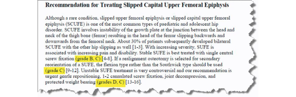
Figure 30.19 A selected paper with grade of recommendation.
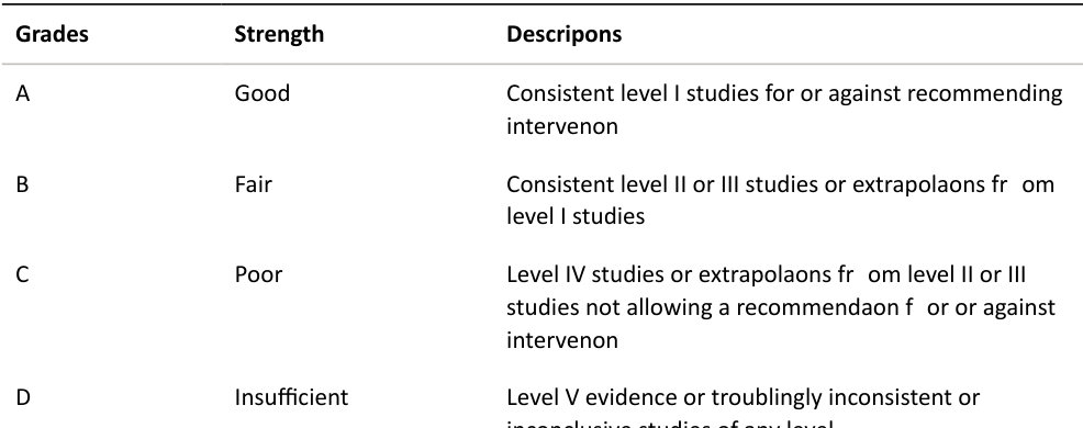
These refer to the grades of recommendation, based on levels of evidence. Several have been described. I follow the one that is recommended by the Oxford Centre for Evidence-based Medicine in which grade A is used for good evidence, grade B for fair evidence, grade C for poor evidence and gradeD for insufficient or conflicting evidence [10] (Table 30.3).
Authors’ note 9: Outcome measures
Outcome measures have become an essential part of many research projects. In fact, a study is considered weak if outcome measures are not used. Having some core knowledge about how outcome measures are developed is important to understand some of the jargon that you may face in the exam (and clinical practice).
Developing an outcome measure involves several processes. This can be summarized as follows [11].
1. Content: (are the contents of the measure relevant to your population?)
Content items are generated in several ways. These items are then gradually reduced based on importance and relevance. The following are considered when items are included, excluded or weighed:
A. Type:
i. Clinician-based outcome measure (CBOM).
ii. Patien t-based outcome measure (PROM).
B. Scale: what questions makeup the outcome? How are they scored?
C. Interpretation: do higher scores indicate a better outcome?
2. Methodology: this involves assessing validity, reliability and responsiveness.
A. Validity: does it measure what it is supposed to measure?
i. Construct validity: quantitative assessment of validity.
1. Divergent: two measures do not correlate highly if they measure different things.
2. Convergent: two measures have a high correlation with each other when they measure the same thing.
Outcome measure must show both convergent and divergent validity evidence for construct validity, but neither alone is sufficient for establishing validity.
ii. Content validity (face validity): are the contents comprehensive and relevant?
This is established by content experts: clinicians and/or patients.
iii. Criterion validity: correlation with golden standard.
1. Predictive validity: ability to predict the future state of health, e.g. patients with low score will do badly.
2. Concurrent validity: accurately predict current state of health when compared with other measures.
B. Reliability: measure the condition the same way every time.
i. Internal consistency: how consistent are the questions in measuring the same outcome; that is why there are several questions to measure a single dimension.
ii. Reproducibility: produce the same results when there are no changes.
1. Intra-observer (test–retest): reproducibility when used on the same patient on two different occasions (provided no changes inpatient condition).
2. Inter-observer: agreement between two or more observers using the same outcome on the same patient at the same time.
C. Responsiveness: ability of the measure to change as the status of the patient changes.
3. Clinical utility:
APa tien ts’ friendliness (acceptability): easy to complete by patients clear questions, easy to understand, does not take time, etc.
B. Clinician friendliness (feasibility): easy to use and administer, does it need licensing or special sotiw are, does it cost, etc.
Table 30.3 Grades of recommendation.
References
1. Wright JG. A practical guide to assigning levels of evidence. J Bone Joint Surg Am. 2007;89(5):1128–1130.
2. Phillips Bet al. Levels of Evidence (March 2009), Oxford Centre for Evidence-Based Medicine 2009
[cited 2012; available from: www.cebm.net].
3. Harbour R, Miller J. A new system for grading recommendations in e vidence-based guidelines. BMJ.
2001;323(7308):334–336.
4. Alshryda S, Huntley J, Banaszkiewicz P. Chapter 1: Introduction to evidence-based practice . In H
Alshryda, JS Huntley, P Banaszkiewicz (Eds.), Paediatric Orthopaedics: An Evidence-Based Approach to
Clinical Questions , Cham: Springer; 2016: 51–75.
5. Howick J, et al. The 2011 Oxford CEBM Evidence Levels of Evidence (Introductory Document). Oxford
Centre for Evidence-Based Medicine. www.cebm.net/index.aspx?o=5653. 2011.
6. Sibbald B, Roland M. Understanding controlled trials. Why are randomised controlled trials important?
BMJ. 1998;316(7126):201.
7. Roland M, Torgerson DJ. What are pragmatic trials? BMJ. 1998;316(7127):285.
8. Wright J, Eastwood DM. Clinical surveillance, selective or universal ultrasound screening in DD HIn H
Alshryda, JS Huntley, P Banaszkiewicz (Eds.), Paediatric Orthopaedics: An Evidence-Based Approach to
Clinical Questions , Cham: Springer; 2016.
9. Goel MK, Khan naP, Kishore J. Understanding survival analysis: Kaplan-Meier estimate Int J Ayurveda
Res. 2010;1(4):274–278.
10. Grades of Recommendation Oxford Centre for Evidence-based Medicine. 2009. Available from:
www.cebm.net/?o=1025.
11. Suk M, Hanson BP, Norvell DC, Helfet SL (Eds.). AO Handbook. Musculoskeletal Outcome Measures and Instruments. Basel: Thieme; 2004.
Section 6