Chapter 26 Biomechanics
Introduction#
The stress–strain curve is a triple A-list subject. It always seems to be asked in viva examinations and is a definite top 10 core basic science question. In recent years this topic has been reinvented as it was becoming too predictable. We make no apologies for including the question in all of its various guises.
Structured oral examination question 1#
Stress–strain curve
Can you draw the stress–strain curve for stainless steel?
Drawing is a vital component of the FRCS (Tr & Orth) Exam. A candidate is expected to illustrate to examiners what they are describing to aid discussion and inform techniques. Drawing also helps a candidate deal with the competency-level questions efficiently and accurately, gaining extra timet o deal with the higher-order thinking questions, leading to higher scores. The stress–strain curve demonstrates how a material subjected to an increasing tensile load deforms until failure (Figure 26.1). Stress is force over area and has units of Newton per square metre. Strain is change in length over original length; it has no units. It is usually expressed as a ratio or percentage.
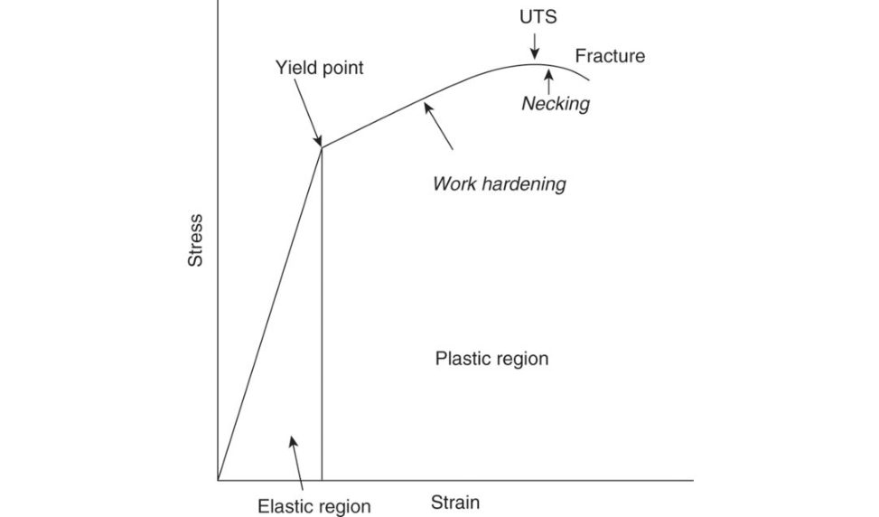
Figure 26.1 Stress–strain curve for a typical metal.
Get this in about strain having no units first. Don’t wait to be asked ‘what are the units of stress?’ by the examiners. Most candidates know it’s a fairly blunt question. 1
How does force change the cross-sectional dimensions of the area it is acting on?
An object understress experiences strain in the transverse direction aswell as the horizontal direction. Transverse strain is usually opposite to longitudinal strain, i.e. as an object gets longer, it gets thinner. As such, force can change the size of the cross-section it is acting upon. However , stress and strain are generally based on the original dimensions of the object.
An initial slightly off-the-wall question can derail a nervous candidate before they have time to setile and hast o be handled with skill. These less-obvious basic science questions are an attempt to move away from conventional book knowledge and force a candidate to apply first principles to problem-solving. The initial section corresponds to elastic deformation. Strain is directly proportional to stress. This is known as Hooke’s law.
What happens to the molecular bonds when in this region of the graph?
The molecular bonds are stretched but not broken. The gradient, i.e. steepness, of the straight line correlates to the material’s resistance to deformation. This is called Young’s modulus of elasticity . The higher the Young’s modulus of elasticity , the smaller the deformation produced for a given load. This here is the yield point, which is the maximum stress up to which a material undergoes elastic deformation. The yield point is the point on the stress strain curve that indicates the limit of elastic behaviour and the beginning of plastic deformation. The non-linear section of the s tress–strain curve corresponds to plastic deformation. The deformation is permanent and if the stress is removed, strain is not completely recovered and the material does not return to its original state.
What happens to the bonds?
Molecular bonds are broken, and the molecules move too far apart to return to their original positions. The ultimate tensile strength is the maximum stress that the material can sustain before fracture. The fracture point is where the material eventually fails. Stress at the fracture point can be slightly less than the ultimate tensile strength because the latter can cause the material to neck, which reduces its cross-sectional area and therefore the force required to fracture. The area under the stress–strain curve represents the energy absorbed per unit volume of the material. It therefore indicates the energy absorbed by the material to failure. This is called toughness. A tough material takes a lot of energy to break it. Comparing two forces acting on two surfaces can be misleading because this does not take into account the size of the cross-section. Stress indicates the intensity of force acting on a section. As such, it is a fairer comparison of loads acting on different surfaces.
You seem to be changing around and mixing up stiffness and strength. What exactly do you mean by these terms?
Stiffness is s tress–strain while strength is the load required to break a material and depends on plastic deformation. Imprecise answer. Stiffness and strength are terms often used interchangeably, but they are distinct mechanical properties. Stiffness is defined as the slope of a force versus displacement graph. Strength is an imprecise term and represents the degree of resistance to deformation of a material. A material is strong if it has a high ultimate tensile strength.
Are you sure?
The steeper a stress–strain curve, the stiffer the material. The less steep the curve, the more flexible the material. The slope of the stress–strain curve is the elastic (Y oung’s) modulus of the material. Mechanical testing measures force on a construct that could consist of bone, ligament and possibly fixation device (plate) and the data obtained relates to properties of the construct as a whole. This is what engineers test in real life. Force and displacement are normalized for an individual material into stress and strain. Force and displacement data will vary if the specimen dimension changes, even if it is from the same material. That is why we normalize force with its cross-section and displacement with its gauge length to arrive at stress and strain. Try to understand rather than rote learn your biomechanical definitions otherwise with imprecise terminology you can get drawn into semantics and end up losing marks.
What is the difference between hardness and toughness?
Hardness describes a material’s resistance to localized surface plastic deformation, eg. scratch or dent. Hardness is not a basic mechanical property, but instead derived from a combination of other material properties, eg. stiffness and strength. Hardness determines the wear resistance of a material. Under the same loading conditions, a harder material has a greater wear resistance than a softer material. Toughness is a material’s ability to absorb energy up to a fracture. Toughness is derived from both strength and ductility of amate rial.
So why is hardness important?
It has great relevance when considering bearing surfaces and wear with implants.
Basic science applied to clinical relevance.
Structured oral examination question 2#
Stress–strain curve
Stress–strain curve – label all the points, axis and nomenclature and describe what the areas underneath signify. What is hardness?
The x-axis represents strain, which is change in length over original length. It has no units. The y-axis is stress, which is force per unit area applied and has the units Newton per square metre (N/m2). The area under the stress–strain curve up to the elastic limit depicts the modulus of resilience (MR), which signifies the ability of material to store or absorb energy without permanent deformation. The whole area under the complete stress–strain curve represents the energy absorbed by the material to failure. This is known as the modulus of toughness, which shows the ability of a material to absorb energy up to fracture. The Young’s modulus can be determined from the gradient of the line in the elastic portion of the stress–strain graph. Hardness is a surface property of a material. It is the ability of a material to resist scratching and indentation on its surface. It has no association with the s tress–strain curve.
How does the Young’s modulus differ for isotropic and anisotropic materials?
Differentiating between isotropic and anisotropic materials is factual and rote-learned. The examiner has linked mechanical properties to Young’s modulus of elasticity to test whether a candidate is able to demonstrate a more advanced level of understanding. An isotropic material behaves identically, irrespective of the direction of applied force. Examples include most orthopaedic metals, polymers and woven bone. The Young’s modulus of elasticity will be constant in all directions the force is applied to the material. With an anisotropic material the Young’s modulus varies depending on the direction of loading Examples include cortical bone, ligaments. We have the yield point here, which is the start of plastic deformation, and the ultimate stress, which is the maximum stress the material can withstand.
Hold on; there are lots of different points on the graph that you haven’t mentioned ( Figure 26.2a).
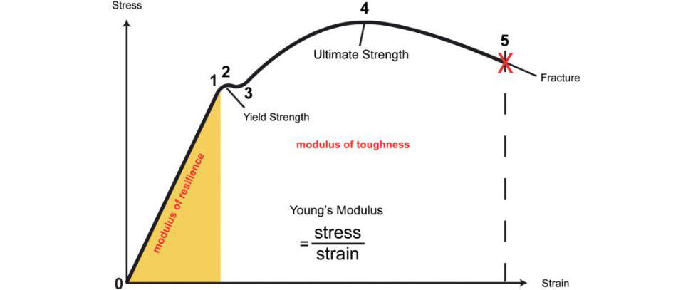
Figure 26.2a Stress–strain curve. Various points on graph include: 1, proportional limit; 2, elastic limit; 3, yield point; 4, ultimate tensile strength and 5, failure.
The point separating the elas tic region and the plastic region is often difficult to identify in the curve. The usual conventionist o define the yield strength, which is the intersection of the curve with a straight line parallel to the elastic deformation of 0.2% on the strain axis.
There are three points on the graph that in some materials are very close to each other and often difficult to differentiate. These are2: 1. Proportionality limit The stress at which Hooke’s law is no longer obeyed. 2. Elastic limit If the stress slightly exceeds the proportional limit, the stress–strain curve is no longer linear but the material may still respond elastically. The curve tends to bend and flatten out. This continues until the stress reaches the elastic limit. The elastic limit is the stress at which permanent deformation is seen and beyond this point the deformity will not completely recover if the force is removed. 3. Yield point The point in the stress–strain curve at which the curve levels off and plastic deformation begins to occur. What is the yield point and how does it differ from the elastic limit?
Some textbooks describe the yield point as very fractionally la ter in the curve than the elastic limit. So the elas tic limit is the point at which deformations tops being entirely reversible and the yield point is the point at which the material will have an appreciable elongation or yielding without any increase in load. However, the two values are virtually inseparable for most materials.
What is the difference between (offset) yield stress and yield point3?
The yield point is that point at which the material starts to undergo plastic deformation. As it is often difficult to pinpoint the exact stress at which plastic deformation begins in some materials, the (offset) yield stress is taken to be the stress needed to induce a specified amount of permanent strain, typically 0.2%. To confuse the issue some engineering textbooks define the yield point as the (offset) yield stress.
What do we mean by the upper and lower yield point (Figure 26.2b)?
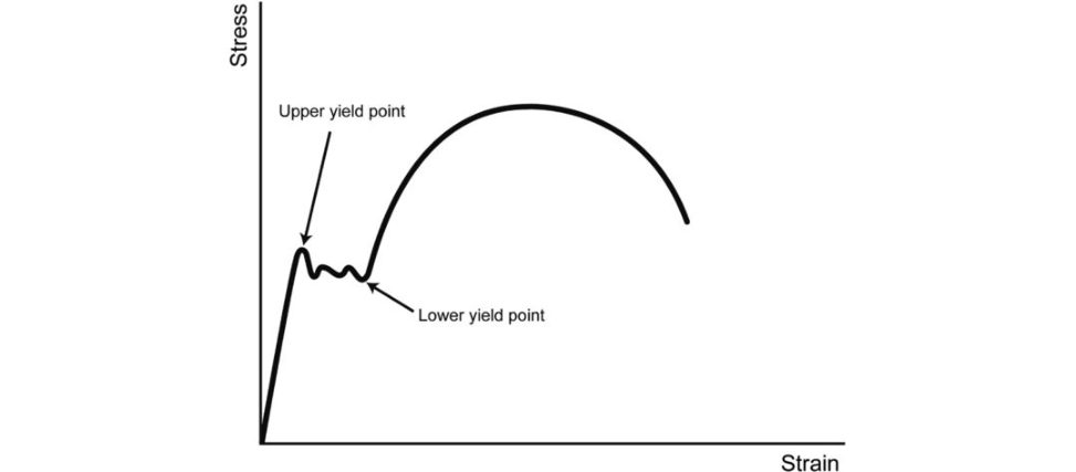
For certain materials, especially low-carbon steel alloys, the stress–strain curve produces both an upper yield point and a lower yield point. A distinctive ripple pattern following the upper yield point is seen and associated with non-homogeneous deformation. The upper yield point is the maximum stress at which deformations tarts. A fairly dramatic drop is then observed in the stress to the lower yield point, although the strain continues to increase. Eventually the material is strengthened by this deformation and the stress is increased with further straining (strain hardening). The phenomenon is thought to occur due to dislocations occurring in the material. Materials lacking this mobility, for instance by having internal microstructures that block dislocation motion, are usually britile and dont have separate upper and lower yield points.
Figure 26.2b Upper and lower yield points on stress–strain curve.
What is happening at the yielding, strain hardening and necking stage of plastic deformation?
I am not completely sure. This is not well explained in most revision FRCS (Tr & Orth) textbooks. For score 8 candidates
The plastic region consists of different parts that are (1) yielding, (2) strain hardening and (3)
necking.
Once the elastic limit (yield point) is passed, the material will undergo considerable elongation
(yielding) with litile or no increase in stress. This is indicated by the flatness of the stress–strain graph region in the plastic region. When the material is in this state it is often referred to as being perfectly plastic.
Strain hardening is where the plastic deformation increases a material’s resistance to further deformation. It occurs due to the material undergoing changes in its atomic and crystalline structure.
Latice defects occurring in the material become too much in number and they restrict each other’s movement. Essentially traffic jams have been created that obstruct movement of latice defects .
An example is cold working of metal alloys. Strain hardening increases the yield point at the expense of lower ductility and toughness. Thus, a material that has received prior deformation will be stronger than an undeformed material.
In the region after the ultimate strength point, stretching occurs with an actual reduction in the stress. This is a result of necking or waisting in the material, whereby the cross-sectional area is reduced.
Although the stress the material can withstand is reduced after the ultimate strength point, this is not due to any loss of material strength but due to the reduction incr oss-sectional area of the bar. If the cross-sectional area of the narrowest part of the neck is used to calculate the stress, then the true stress-strain curve is obtained.
Structured oral examination question 3#
Stress–strain curve
Draw me the stress–strain curves for materials used in THA (Figure 26.3a). What is the stress–strain curve for ceramic, UHMWPE and stainless steel?
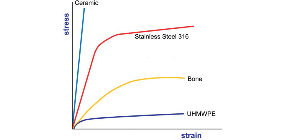
Sharp intakes of breath if you haven’t read up beforehand, but relatively easy if you have worked through a pre-exam answer. Ceramic is a very britile material while UHMWPE is plastic Stainless steel is ductile. Ductility is a measure of the ability of a material to be drawn out that is plastically deformed, before failure. Stainless steel 316 is moderately strong, tough and a highly ductile material (this allows bending before catastrophic failure).
Figure 26.3a Stress–strain curve for materials used in THA.
What is happening with this graph (Figure 26.3b). Can you interpret it for me?
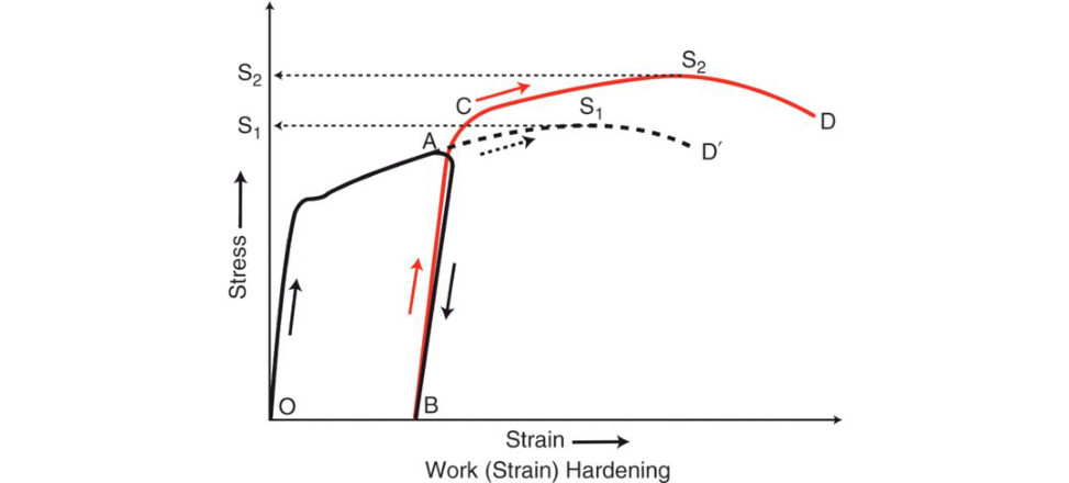
Figure 26.3b Strain hardening of a material.
This is demonstratings train hardening of a material. When loaded, the strain increases with stress and the curve reaches the point A in the plastic range. If at this stage, the specimen is unloaded, the strain does not recover along the original path AO, but moves along AB. If the specimen is reloaded immediately, the strain increases with stress from B to A but via another path (the slope of stress–strain line is steeper indicating that the material has got stiffer than before) and reaches the point C, after which it will follow the curvature if loading is continued. If the specimen would not have been unloaded, after point A, the stress–strain curve would have followed thed oft ed path ADʹ. Comparison of paths AC Dand ACDʹ shows that due to cold working (plastic deformation), the yield strength and ultimate strength have increased. Ultimate strength increased from S1 to S2. Since the ductility has decreased the work to failure on reloading also decreases. Thus strain hardening reduces toughness.
What about UHMWPE used in joint arthroplasty. What are its properties?
UHMWPE has low friction and high impact strength, excellent toughness and low density, ease of fabrication, bio compatibility and bio stability. Its major drawback is wear. There have been changes in the way PE is manufactured in recent years. Gamma irradiation in air is bad due to generation of free radicals which can become oxidized and ...
That’s fine, we don’t need to go there.
Structured oral examination question 4#
Stress–strain curve
Stress–strain curve of different materials ceramicSS, plastic, bone, ligament), how are they different (Figure 26.4)?
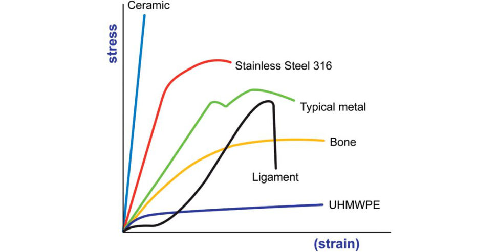
Figure 26.4 Stress–strain curves of different materials.
Essentially this is describing and interpreting the s tress–strain curve for britile (ceramic), ductile (CoCr) and plas tic elas tic materials. Bone (mostly britile but with alit ile plastic deformation before failure) doesn’t neatly fit into one of the above categories. Leading on from bone the examiners may choose to throw into the discussion isotropic versus anisotropic material properties. Be careful with bone as the stress–strain curve is different for cortical and cancellous bone.
Describe how each material behaves when loaded.
Candidates should be able to discuss the elastic and plas tic regions of the graph and how they differ between the various materials. This question is a different way of essentially testing the factual knowledge of the stress–strain curve.4
How is the mode of failure (fracture) different between britile and ductile materials ?
Materials fracture by a process of crack initiation and propagation. All materials are rough and contain defects and cracks at the microscopic level. Crack progression in abri tile fracture is associated with litile plastic deformation whereas ductile fracture involves significant plastic deformation. Abri tile material fails suddenly, soon after the yield point.
The appearance of abri tile fracture is characterized by a clearly defined fracture surface generated across the material.
With a ductile fracture there is considerable deformation after the yield point that results in a characteristic ‘drawn out’ appearance.
Structured oral examination question 5#
Stress–strain curve
Can you drawout the stress-strain curve – label all the points, axis and areas of interest (Figure 26.5a)? What happens at the yielding, strain hardening and necking regions of the graph (see above)? Stress–strain curve of materials with three different moduli of elasticity . Pick three items from a display in front of me that match those stress–strain curves. Describe their material properties (ceramic/bone/ligament) (Figure 26.5b).
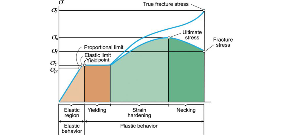
Figure 26.5a Stress–strain curve diagram for ductile material (stainless steel).
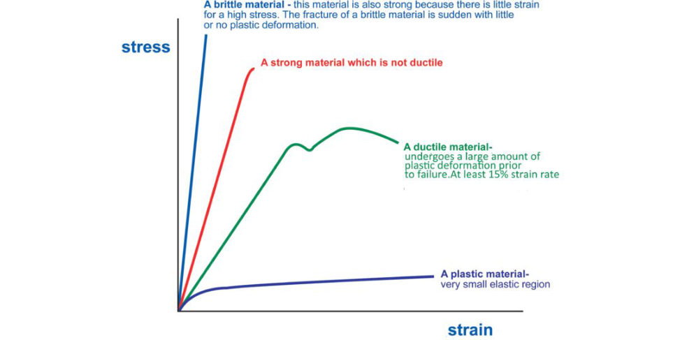
Figure 26.5b Stress–strain curve, different materials.
Abri tile material is one that exhibits a linear stress–strain relationship up to the point of failure. It undergoes elastic deformation only with liti leto no plastic deformation. Characterized by the fact rupture occurs without any noticeable prior change in the rate of elongation. The classic example to mention is ceramic Other examples would include PMMA and glass (Figure 26.5c). Although cortical bone exhibits some plastic deformation it behaves more like abri tile material than a ductile material. It deforms slightly before failure or fracture. Cortical bone displays anisotropic behaviour with its elastic modulus depending on the direction of loading. It is also viscoelastic, with the s tress–strain curve varying depending on the rate of loading. Ligament is also viscoelastic. The toe region of the stress–strain curve is seen predominantly in ligaments and tendons. It denotes a non-linear elastic phase. Initially , a large distance (strain) is travelled under minimal stress as the crimped fibres straighten out. The characteristic shape is produced by the increase in the number of collagen fibrils resisting the strain as the slack fibrils are straightened and stretched, reducing the crimp pattern. Once all the collagen fibrils are straightened and stretched the slope is more orless constant (linear region).
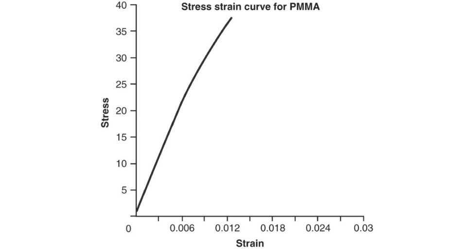
Figure 26.5c Stress–strain curve for PMMA. Essentially britile with litile plastic deformation before failure.
What about the stress–strain curve of cortical vs cancellous bone (Figure 26.5d)?
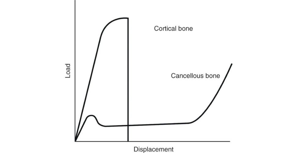
The compressive stress–strain curve for cancellous bone shows an initially shorter elastic segment (lower yield point) and has a lower stiffness (< 10% that of cortical bone). Upon reaching the yield point, however, cancellous bone has a very long plastic phase. This phase represents the progressive fracture and collapse of the cancellous trabecula. Once trabecular debris fills the marrow spaces and the cancellous bone compacts, the curve once again turns upward, illustrating the resulting increased stiffness. This prolonged plastic deformation period explains why the total energy absorbed by cancellous bone under compression can exceed that of cortical bone.
Figure 26.5d Compressive stress–strain curve cortical vs. cancellous bone. There is a prolonged plateau in cancellous loading representing the collapse of trabeculae.
Structured oral examination question 6#
S-N curve
S-N curve (Figure 26.6a). What is this, what does it mean and label the axis? Relate this to both THA and TKA.
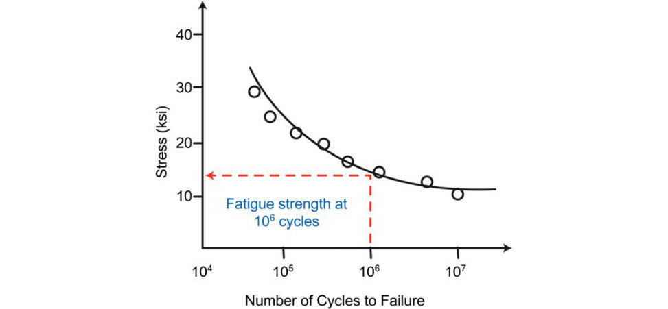
Figure 26.6a S-N curve. Specimens are tested in a series of decreasing stress levels until no failure occurs within a selected maximum number of cycles. The nearly horizontal portion of the curve defines the fatigue or endurance limit. If the applied stress is below the endurance limit of the material, the specimen is said to have an infinite life.
Fatigue properties of amate rial are normally demonstrated on an S-N curve. Stress on the y- axis is ploft ed against number (n) of cycles (millions) on the x-axis. At stresses below the endurance limit, a material can be cycled endlessly without experiencing failure. The higher the peak stress produced in a given cycle of loading and unloading, the fewer cycles that can be sustained before failure. Fatigue or endurance limit is normally defined at 106 or 107 cycles. Some metals such as aluminium do not have a fatigue limit.
So, what is the difference between fatigue strength and fatigue limit?
For some materials the S-N curve becomes horizontal at higher n values or there is a limiting stress level called the fatigue limit (some times called endurance limit) below which fatigue failure will not occur. For other materials (e.g. aluminium, copper, magnesium) they do not have a fatigue limit, the S -N curve continues its downward trend at increasingly greater n values. As such, fatigue will ultimately occur regardless of the magnitude of the stress. For these materials, the fatigue response is specified as fatigue strength, which is defined as the stress level at which failure will occur for some specific number of cycles (e.g. 107, 108).
Clinically, THA operate above the endurance limit, while TKA operate at the endurance limit, especially the polyethylene component, predisposing the latter to fatigue failure.
It is important to avoid creating an y scratches or dents that can act as stress raisers and so reduce the fatigue properties of anim plant.
Fatigue failure in orthopaedic implants is much less common with improved materials and processing.
Mechanical requirements of arthroplasty materials include a high yield point and endurance limit, modulus of elasticity that is similar to bone and wear resistance.
A concern is high and frequent loads on the hip joint. It is estimated around 1 million cycles per year occur at the hip that could potentially lead to fatigue failure.
What do we mean by notch sensitivity?
Notch sensitivity is the extent to which the sensitivity of amate rialto fracture is increased by the presence of a surface inhomogeneity, e.g. cracks and scratches. The initials tress concentration associated with a crack is too low to cause a fracture but may be sufficient to cause slow growth of the crack. Eventually the crack becomes sufficiently deep so that the stress concentration exceeds the fracture strength and sudden failure occurs. In britile materials a crack grows to a critical size from which it propagates right through the structure in a fast manner, whereas with a ductile material the crack keeps geting bigger until the remaining area cannot support the load and a ductile failure occurs. A notch causes nonuniform stress flow lines.
Stress–strain curve for a viscoelastic compound (Figure 26.6b). What is this? Explain viscoelasticity . Discuss creep/hysteresis/stress relaxation.
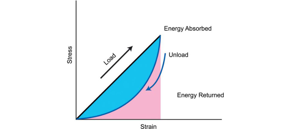
Figure 26.6b Viscoelastic materials exhibit a timed ela y in returning the material to original shape. Some energy is lost. Loading unloading curves are different.
Most biological tissues are viscoelastic (eg. tendon, ligament, bone, articular c artilag e).5 A viscoelastic material exhibits stress–strain behaviour that is time and rate dependent i.e. the material deformation depends on the load and its rate and duration of application. A viscoelastic material is intermediate in properties between an elastic solid (that stores all the energy used to deform it) and a viscous liquid (that dissipates all the energy used to deform it by flow). Viscoelastic materials demonstrate four properties: 1. Stress relaxation. 2. Creep. 3. Hysteresis. 4. Strain rate sensitivity . The first three are specific mechanical properties that are present in viscoelastic materials, while the fourth property relates to a material being more rigid when it is rapidly loaded. A viscoelastic material continues to deform when a constant stress is applied to it. This continued deformation is creep. The creep rate decreases with time. If a viscoelastic material is held at a constant strain, the stress will decrease with time. This is called stress relaxation Therefore, stress relaxation is the inverse of creep. Stress relaxation time decreases with time. A viscoelastic tissue does not follow the same path on a stress–strain graph. This is called hysteresis. The area under the initial loading phase represents the energy used to deform the material. The area used for recoil is the area under the unloading curve, and isless than the energy used to deform the material. The area between the two curves is the energy used to change the shape of the material (lost as heat) between loading and unloading. As a result, further energy is required to continue the loading and unloading cycles. This property allows viscoelastic materials to act as shock absorbers.
Viscoelastic materials are usually stiffer, stronger and tougher when loaded at a higher strain rate.
This is called strain rate sensitivity and is duet o the fact that the material isn’t as quick to deform at a higher strain rate.
There are various slightly differently worded definitions of cr eep/hysteresis/stress relaxation in the textbooks. Just learn one standard definition that you are comfortable with and stick with it.
Can you give me some everyday examples of creep, stress relaxation?
The handle of a heavy shopping bag gets longer and thinner as you walk home. This is creep, a material stretching out over time when subjected to a constant deforming force. An example of stress relaxation is when a rubber bandis wrapped around a newspaper for an extended period of time.
What about strain rate sensitivity?
Sorry, no. Blu tack.6
Structured oral examination question 7#
Draw stress–strain curve and mark the events. Draw the curve for a ductile material. Viscoelastic properties, draw the curves for these.
Usual standard question Remember ductility is the ratio of ultimate strain to yield strain.
Can you describe the biomaterial behaviour of material A, B and C (Figure 26.7a)?
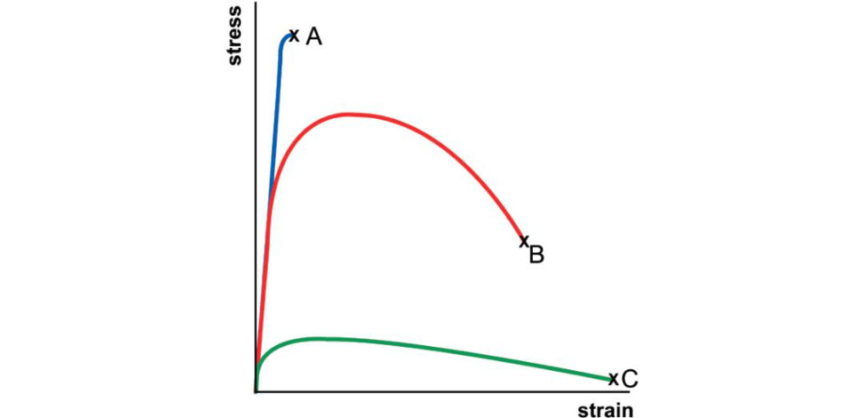
Figure 26.7a Stress–strain curve for various materials.
A has high strength, low ductility and low toughness. It is the strongest material. B has high strength, high ductility and high toughness. C has low strength, high ductility and low toughness. It extends or stretches the most.
What do you mean by strength, ductility and toughness?
Strength is a somewhat imprecise term, but relates to the degree of resistance to deformation of amate rial. A material is strong if it has a high ultimate tensile strength. Toughness is the amount of energy per unit volume that a material can absorb before failure. When comparing britile and ductile materials with the same ultimate strengths, the britile material isless tough as it has less area under the stress–strain curve. Ductility is thea mount of plastic deformation that occurs before failure.
What do we mean by creep, stress relaxation and hysteresis? Can you drawout the relevant graphs (Figure 26.7b–26.7d)?

Figure 26.7b, c and d Candidate drawings of creep, stress relaxation and hysteresis.
See previous questions above. Figure 26.7b, c and d. Candidate drawings of creep, stress relaxation and hysteresis. Talk as you draw making sure your explanation is spot on for accuracy.
What about elastic materials?
Elastic materials do not exhibit energy dissipation or hysteresis as their loading and unloading curve is the same. Indeed, the fact that all energy due to deformation is stored is a characteristic of elas tic materials. Furthermore, under fixed stress elastic materials will reach a fixed strain and stay at that level. Under fixed strain, elastic materials will reach a fixed stress and stay at that level with no relaxation.
Structured oral examination question 8#
Stress–strain curves for different materials
Materials – what is steel and what is titanium? Stress–strain curves for a variety of different materials.
What is HA, why is it on a Ti stem, how is it put on a Ti stem?
What is stainless steel?
Initials tress–strain curve questions can be a leadin (or prop) to go on and discuss biomaterials. Steel is normally comprised of carbon andiron. If chromium is added it forms an oxide layer on the outer surface that protects it from corrosion – these alloys are stainless steel. The most common stainless steel in orthopaedics is 316 L. The number 316 refers to 3% molybdenum and 16% nickel added to a normal alloy of iron, carbon and chromium. The letter L indicates a low carbon content < 0.03%. Molybdenum reduce spiting corrosion. Carbon content improves corrosion resistance, but too high a level weakens the alloy. It is usually annealed, cold-worked or cold-forged for increased strength. It is ductiles tiff and cheap. Its use in arthroplasty surgery has been limited as Ti and CoCr alloys have better wear and corrosion resistance and lower stiffness. R elativ ely low biocompatibility and technical difficulties with MRI. Implant stainless steel contains nickel, which improves corrosion resistance and increases fatigue strength and toughness. However, nickel can cause allergy and there have been recent attempts to reduce its content inSS. Some newer SS contains a high nitrogen content that makes it stronger and more resistant to localized corrosion. Titanium is extremely strong, has half the stiffness of cobalt chromium and can osseointegrate with bone. It has excellent biocompatibility . Undergoes self-passivation to form an adherent oxide layer which decreases corrosion. High yield strength. It has poor wear characteristics and a high coefficient of friction, making it unsuitable for use as an articulating bearing surface in THA. Notch-sensitiv e and rough. The most commonly used orthopaedic titanium alloy is titanium 64. The numbers refer to alloying elements aluminium (6%) and vanadium (4%). Calcium hydroxyapatite is the mineral phase of bone.
HA is used as an adjuvant surface coating on prosthetic cup ors tem surfaces that are usually made of a titanium alloy (TiAlV).
Why is this?
When compared to cobalt chromium titanium demonstrates a 33% increase inbond strength. The modulus of elasticity of titanium is closer to bone, resulting inlesss tress shielding and bone resorption. As such titanium alloy is the preferred metallic substrate of choice. In addition, although HA can be used on both porous-coated ingrowth and grit-blasted ongrowth femoral implants, for the most part it is mainly used on anon growth surface. The candidate is either very knowledgeable or digging a hole for themselves.
What is the reason for this?
Porous ingrowth surfaces appear to have a greater inherent initial stability which encourages biological fixation. Although HAu sage depends somewhat on philosophy, many surgeons believe it has only a limited early role for an ingrowth surface and potential disadvantages outweigh benefit. The situation is different with grit-blasted implants. Fixation occurs by bony ongrowth on the implant surface, which requires a more extensive area of coating to secure the implant as this is a weaker method of fixation. As such HA is added to improve early stability, reduce micromotion in the immediate postoperative period and accelerate bone ongrowth onto the prosthesis surface. There is some evidence that HA coating works best on plasma-sprayed ongrowth surfaces rather than grit-blasted ongrowth surfaces. Odds even with this answer.
Why do we use grit-blasted stems if ingrowth stems appear to have a better chance of initial stability and obtaining osseointegration?
The manufacturing process for porous ingrowth stems can result in diminished fatigue strength properties. This could result in implant failure over time.
How is HA put on a Ti stem?
HA deposition is often achieved through the plasma spray technique, which is performed at high temperature (15,000°C) and under vacuum, by projecting HA particles on to the metallic material at a speed of 300 m/s. The metallic substrate has a rough surface to promote adhesion. The other manufacturing method achieves HA deposition by electrochemical means, although it appears that the plasma spray technique is associated with improved bone ongrowth.
H A is an osteoconductiv e agent that allows for more rapid closure of gaps. Its surface readily receives osteoblasts and thus provides a bidirectional closure of gaps (i.e. bone to prosthesis and prosthesis to bone), which clinically shortens the timet o biological fixation.
The optimal thickness of hydroxyapatite is 50–75 μm. Thicker coatings have been reported to delaminate off the prosthetic interface.
Is there much difference in the clinical outcome or survivorship between HA-coated stems and uncoated stems.
From what I understand of the literature there isn’t much evidence to support any difference in outcomes in terms of improved hip function radiological assessment or survivorship.
What radiological outcomes are you assessing?
Radiological outcomes included the presence of endosteal condensation (spot w elds) and the presence of radioactive lines. Endosteal condensation is considered a sign of endosteal bone ingrowth on the surface of the femoral stem and suggests that femoral stem fixation is optimal. Radioactive lines indicate femoral stem instability and are considered a sign of micromotion and femoral stem loosening. Use of HA-coated femoral stems has several disadvantages. These include high cost and the potential for delamination of the HA coating. HA particles delaminated from the stem surface may induce osteolysis either by stimulating bone loss or by migration to the joint space producing third-body wear.
Can you please draw the stress–strain curve for steel?
The stress–strain curve for stainless steel is typical of that for a ductile material. The question may just require a simplified stress–strain diagram to be drawn as for a ductile material (Figure 26.8) or require the full-blown stress–strain diagram to be drawn out with the various regions and points explained (Figure 26.2a).
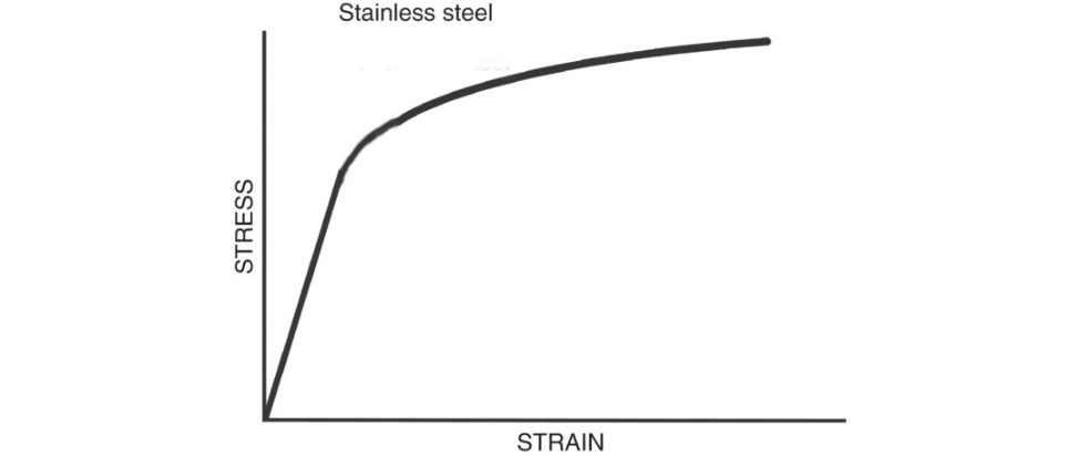
Figure 26.8 Simplified stress–strain curve for steel.
The stress–strain curve for ligament vs. tendon?
Ligaments and tendons are predominantly made up of collagen. As such their stress–strain relationship is very similar to that of collagen. There are a few minor differences in the stress–strain curve between ligament and tendon. This is mainly in the toe region of the curve. It takes slightly longer for a ligament to reach the elastic part of the graph as its collagen fibres are more wavy, less unidirectional and less w ell-structured compared to tendon. The slightly larger content of elastin in ligaments makes them less stiff and slightly weaker than tendons. The toe-in region represents ‘uncrimping’ of the crimp in the collagen fibrils. Because it is easier to stretch out the crimp of the collagen fibrils, this part of the stress–strain curve shows a relatively low stiffness. As the collagen fibrils become uncrimped, the collagen fibril is being stretched, which gives rise to a stiffer material. As individual fibrils within the ligament or tendon begin to fail, damage accumulates, stiffness is reduced and the ligament/tendon begins to fail.
Structured oral examination question 9#
Free body diagrams: elbow
Quite a large part of biomechanics involves drawing and explaining around free body diagrams (FB DIn the good old days of the past, if the examiners wanted topass a candidate they would ask them to draw a free body diagram of the elbow. This is probably the easiest joint for a candidate to drawout and explain.
Most candidates should breeze through this question with ease.
If examiners were unsure of a candidate they would ask them to draw a FBD of a hip and see how they got on. If a candidate managed to give a reasonably good account of themselves this was great and the candidate was passed with a move on to the next question. If a candidate managed to botch the answer up, the examiners’ initial concerns were being realized. The examiners would then begin to unravel the candidate by asking them to drawout another FBD of the hip, but this time with a person holding a stick. This was make or break for the candidate to redeem themselves, but if they messed up again then a couple more FBDs of a person holding a suitcase in one hand, or a suitcase in both hands would usually be enough to sink them.
If the examiners were keen to fail a candidate for whatever reason they would ask them straightup spinal biomechanics. Most candidates will struggle with this and would usually fail miserably. So much for the good old days!
What do we mean by a free body diagram?
This is a method used to illustrate the various forces acting onas tructure such as a bone, and to illustrate how far from a joint or other pivot point these forces are acting. From knowing these forces and distances, the moments of force acting to maintain the structure in static equilibrium can be calculated. FBD show the locations and directions of all forces and moments acting on a body . They are useful for identifying and evaluating unknown forces and moments acting on individual parts of a system in static equilibrium (i.e. sum of forces and moments is zero). They can not be used for dynamic equilibrium.
What are the assumptions made when drawing a free body diagram?
The assumptions made are that7: Bones are rigid bodies. Joints are frictionless hinges. There is no antagonistic muscle action. The weight of the body is concentrated at the exact centre of body mass. Internal forces cancel each other out. Muscles only act intension (no compressive forces).
The line of action of a muscle is along the centre of the cross-sectional area of the muscle mass.
Joint reaction forces are assumed to be compressive only (no tensile forces).
The joint acts only as a hinge (other axes of rotation and translation are ignored).
What do we mean by a joint reaction force?
JRF is the force generated within a joint in response to external forces. It is the vector sum of all forces acting on the joint.
Can you draw a free body diagram of the elbow joint with an object in the hand (Figures 26.9a and 26.9b)?

Figure 26.9a Arm flexed at 90° at the elbow, with wrist and fingers rigid, holding a ball in palm of hand.
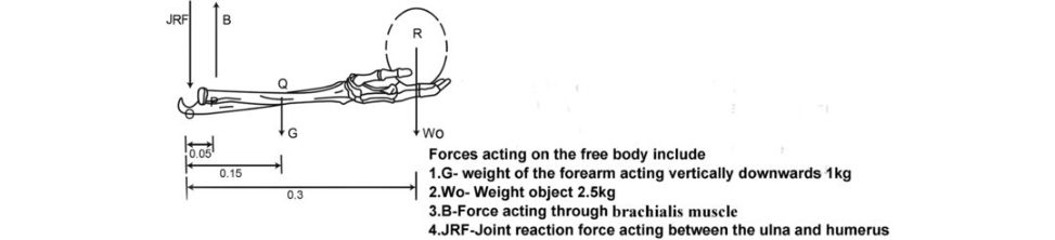
Figure 26.9b Free body diagram showing forearm holding a ball.
Candidates may be straight on asked to draw a free body diagram of a particular joint without the warmup preamble of general free body analysis assumptions (see above). It is reasonable to mention the general assumptions a t the beginning of the viva and then go on to joint-specific assumptions afterwards. The examiners will quickly move a candidate on if they don’t want them to focus on this. My assumptions when drawing the FBD of the elbow are that: The wrist, hand and finger joints are all rigidly fixed. Arm is flexed 90°. Acting as a class III le ver. The moment arm of the biceps/brachialis is shorter than the weight of the forearm. Brachialis and biceps provide all of the flexion force. The force provided by biceps and brachialis is acting vertically upwards.
Elbow fulcrum for the forearm lever.
It is a two-dimensional X–Y plane.
The axis about which an object rotates as the result of a force exerted on the object is called the instantaneous axis of rotation (IAR).
The entire mass of an object is considered to be concentrated at a point called the centre of mass (COM) and does not depend on gravitational field.
Centre of gravity (COG) is the point from which a weight is considered to act and depends on gravitational field.
The centre of mass and the centre of gravity of an object are in the same position if the gravitational field in which the object exists is uniform. In most cases this is true to a very good approximation. It is generally assumed that for most situations C OM = COG. Each joint has specific load interactions because of the particular characteristics of the joint and the muscle actions that cross the joint. Point O is the IAR of the elbow joint. Point P attachment of brachialis on the radius. Point Q is the COG of the forearm. Point R lies on the vertical line passing through the COG of the weight held in the hand. Forces acting on the free body include: 1. G – weight of the forearm acting vertically downwards, 1.5 kg. 2. Wo – weight of object, 2 kg. 3. B – force acting through the brachialis muscle. 4. R – joint reaction force (JFR) acting between the ulna and humerus. Considering the rotational equilibrium of the forearm about IAR, summation of moments about O will be zero. Sum of clockwise (extension) = anticlockwise flexion) moments ∑ M = 0 Wf × 0.15 + Wo × 0.3 = 0.05 × Biceps 15N × 0.15 + 20N × 0.3 = B × 0.05 2.25 + 6 = 0.05B 165N = B (Brachialis force) As the forearm is in translational equilibrium the sum of the forces ∑ F = 0 acting on it is zero. There is no JR Fin the X-axis.
B – G – W – J (JRF) = 0
JRF(J) + 15 + 20 = 165 N
JRF = 165 – 35
JRF = 130 N
Different textbooks have different values for the load carried in the forearm and different distances for P, Q and R. Learn a simplified FBD of the elbow that can be quickly drawn (Figure 26.9c). Some diagrams have only biceps labelled others only the brachilis muscle. With the elbow flexed to 90° by the side of the body, brachialis is the main muscle that maintains this position.
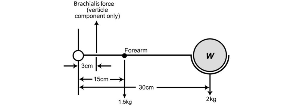
If you are doing very well or very poorly then the examiners may ask you to calculate JR Fon the elbow inextension (Figure 26.9d).
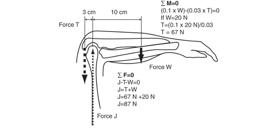
Use the same methods as used for elbow flexion.
Figure 26.9c Candidate 20-second simplified FBD elbow.
Figure 26.9d Joint reaction force on the elbow joint during extension using the same method as that for elbow flexion.
∑ M = 0
(0.1 × W)–(0.03 × T) = 0
If W = 20N
T=(0.1 × 20N)/0.03
T = 67N
∑ F = 0
J–T–W =0
J = T + W
J = 67N + 20 N
J = 87N
For a brownie point, candidates may be asked what type of lever is occurring inflexion and extension. A class 1 lever with elbow extension whereas a class 3 lever with a flexed elbow. The FBD of an extended elbow is approximated to a certain extent in various textbooks in that they show what appears to be a reversed flexed elbow. The elbow is held in 90° of flexion with the forearm positioned over the head and parallel to the ground. In this position, action of the elbow extensors is required to offset the gravitational force on the forearm. It is assumed that triceps is the major extensor and that the force through the tendon of this muscle acts perpendicular to the longitudinal axis of the forearm.
Structured oral question 10#
Hip FBD
The hip joint is somewhere between the elbow and the spine. There are enough scenarios and questions to easily use up 5 minutes of viva time on this topic alone. If a candidate can practise drawing out a standard FBD of a hip in around 20 seconds, then they will create more time to get further on forward with the question chain and sc ore some extra marks.
Can you draw a free body diagram of a hip joint when a person stands on one leg (Figure 26.10a and 26.10b)?
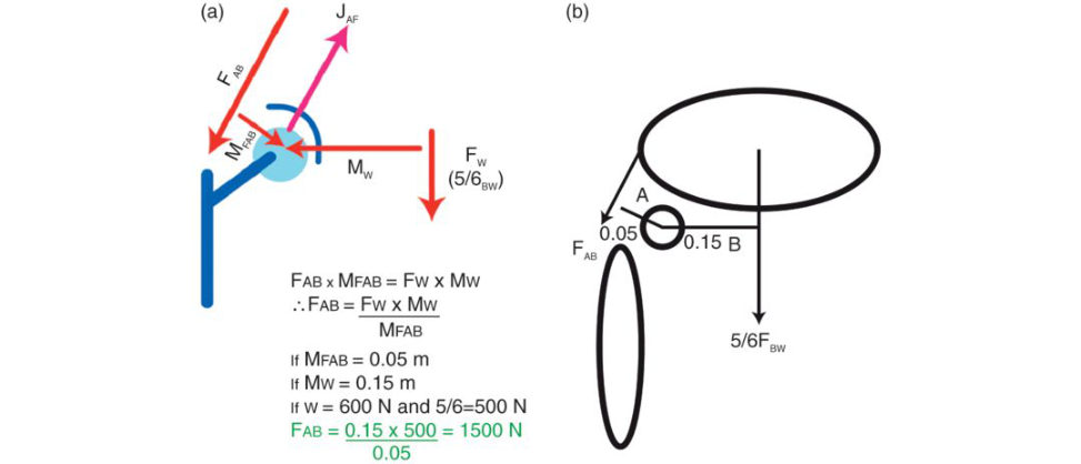
Figure 26.10a and 26.10b Candidate drawing of FBD hip.
Mention general assumptions with FBD first and then the specifics for the hip. We are assuming the: Body is in a single leg stance. Weight of the leg is one-sixth of the total bodyweight. Hip is fixed and the pelvis mobile. Clockwise moment = Anticlockwise moment ∑ M = 0 Sum of moments is zero FAB × MFAB = FW × MW ∴ FAB = FW × MW MFAB If MFAB = 0.05 m If MW = 0.15 m If W = 600 N and 5/6 = 500 N FAB = 0.15 × 500 = 1500 N 0.05
Be careful with the line of action of the abductor muscles. In some textbooks it is assumed they are predominantly acting in aver tical direction while in other textbooks the abductor force is split into My and Mx components. The abductor force is three times closer to the fulcrum (0.05 m vs. 0.15 m). A force triangle is then drawn to calculate the JFR. This is estimated by lengths of the limbs (calculate with scale drawings) or by trigonometry (Figure 26.10c).
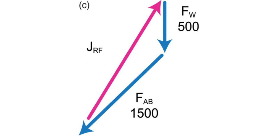
Figure 26.10c A force triangle is drawn to calculate JRF -estimated by lengths of the limbs or by trigonometry JFR = FAB + FW
What class of lever is this?
This is a classI lever between the bodyweight and abductor force.
What happens to the joint reaction force in the hip if the patient has osteoarthritis of the hip and is given a walkingstick in the opposite hand (Figure 26.10d)? Can you draw this out for me?
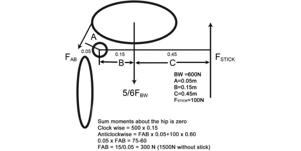
- BW = 600 N
- A = 0.05 m
- B = 0.15 m
- C = 0.45 m
- FSTICK = 100 N
Sum of moments about the hip is zero
Clockwise = 500 × 0.15
Anticlockwise = F AB × 0.05 + 100 × 0.60
0.05 × FAB = 75 – 60
FAB = 15/0.05 = 300 N (1500 N without stick)
Figure 26.10d FBD hip with walkingstick.
What are the properties of a s tick?
Introducing a stick on the opposite side adds another anticlockwise moment. The effect is to lower the bodyweight force and aid the abductors. As the moment arm on the stick is large there is a significant reduction in JRF . The joint reaction force is reduced by 80% with using a walkingstick in the contralateral hand.
How do you calculate the optimum length of shaft. How would a person walk if the stick is too short? And too long?
Apa tien t should stand upright inshoes they would normally use. The elbow should be slightly flexed and shoulders level. The walkingstick should be turned up side down so that the handle is resting on the floor . The distance between the ground and end of the stick should r each to the distal wrist crease (or ulnostyloid joint). The distance between the ground and distal wrist crease is measured as the optimal length of a stick. The method of measuring the distance from the greater trochanter to the ground is not accurate or effective. A number of formulae can be used if a person’s height or arm length is known. If a walkingstick is too short, the patient will stoop orlean to one side throwing the patient off balance. If it is too long, using it can cause shoulder pain and be uncomfortable.
What about carrying a suitcase on the opposite side as the weight-bearing leg. Can you draw this out for me (Figure 26.10e and 26.10f)?
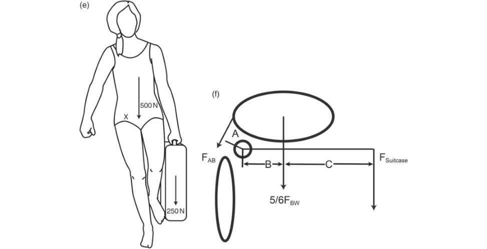
Figure 26.10e and 26.10f FBD with patient carrying a suitcase opposite side of the weight-bearing limb.
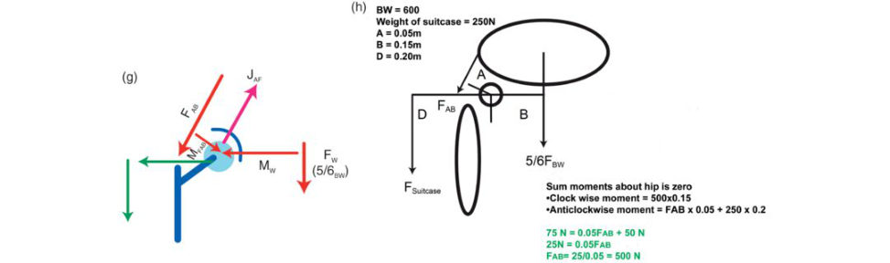
Figure 26.10g and 26.10h FBD with patient carrying a suitcase on the same side as the weight-bearing limb.
Adding a suitcase on the opposite side introduces a clockwise moment which disadvantages/hinders the abductors. This increases the JRF.
BW = 600 N
Weight of suitcase = 250 N
A = 0.05 m
B = 0.15 m
C = 0.45 m
Sum of moments about the hip is zero
Clockwise moment = 500 × 0.15 + 250 × 0.6
Anticlockwise moment = FAB × 0.05
0.05FAB = 75+150
FAB = 225/0.05 = 4500 N
The abductor force that has to be generated is significantly increased by carrying a suitcase in the opposite hand.
Constructing a force triangle to calculate the JRF will show a significantly increased JRF.
What about carrying a suitcase on the same side as the weight-bearing leg. Can you draw this out for me (Figure 26.10g and 26.10h)?
Adding a suitcase on the same side introduces an anticlockwise moment that aids the abductors. The amount of force needed to be generated by the hip abductors is reduced and JRF is reduced. BW = 600 N Weight of suitcase = 250 N A = 0.05 mB = 0.15 mD = 0.20 m Sum of moments about hip is zero
- Clockwise moment = 500 × 0.15
- Anticlockwise moment = FAB × 0.05 + 250 × 0.2
75 N = 0.05FAB + 50 N
25 N = 0.05FAB
FAB= 25/0.05 = 500 N
Despite the extra weight carried, the JRF is reduced by carrying a suitcase in the ipsilateral hand.
What about carrying a suitcase in both hands (Figure 26.10i and 26.10j)?
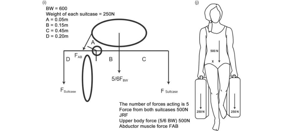
BW = 600 N
Weight of each suitcase = 250 N
A = 0.05 m
B = 0.15 m
C = 0.45 m
D = 0.20 m
The number of forces acting in this situation is 5
Force from both suitcases 500 N
JRF
Upper body force (5/6 BW) 500 N
Abductor muscle force FAB
Sum of moments about hip is zero
- Clockwise moment = 500 × 0.15 + 250 × 0.6
- Anticlockwise moment = FAB × 0.05 + 250 × 0.2
75 N + 150 N = 0.05FAB + 50 N
175 N = 0.05FAB
FAB= 175/0.05 = 3500 N
There is a large clockwise moment arm when carrying a suitcase in the non-weight-bearing side that is not equally balanced by carrying the second suitcase on the weight-bearing side. As such, the hip abductor force required to be generated is high.
Figure 26.10i and 26.10j FBD with patient carrying a suitcase in both hands.
In all the above examples, for simplicity’s sake we have assumed the centre of mass (COM) is unchanged. However, if a person carries a suitcase in the left hand during a right leg stance weight the COM usually shit is towards the left of the person. This additionally increases FAB and JRF. If a person is carrying two suitcases the bodyweight is more balanced, which shitis the C OM closer to the femoral head, thus decreasing the moment arm to the COM so the abductor muscles don’t have to work as hard (less force) to overcome the moment due to the weights leading to a lower reaction force.
What other methods are used to decrease the joint reaction force in the hip joint?
Augmenting the abductors or reducing the bodyweight moment achieves a reduction in the JR FActions that increase the abductor force include: Carrying a suitcase on the ipsilateral side. Lateralization of G T. High offset femoral stem. Actions that have the effect of reducing bodyweight moment: Losing weight. Trendelenberg lurch – shitiing bodyweight nearer to the femoral head, thereby decreasing lever arm. Stick on contralateral side.
Medialization of THA cup (shitis centre of rotation medially thereby decreasing abductor tension).
What actions increase joint reaction?
Valgus neck–shaft angulation – decreases shear across joint.
Structured oral question 8#
Spine
The difficulty with a FBD of the spine is that for a candidate to be at their very best in answering this question the y need to first understand Pythagoras’ theorem.
If a candidate is tight for time the temptation is to go straight to the crux of the question This can create quite a bit of head scratching for most trainees, as it is many years since they studied A-level maths.
For the loading conditions shown, calculate the erector spinae muscle force FM and the compressive and shear components of joint reaction force (FJC and FJS at the L5/S1 vertebrae red square) (Figure 26.11a).
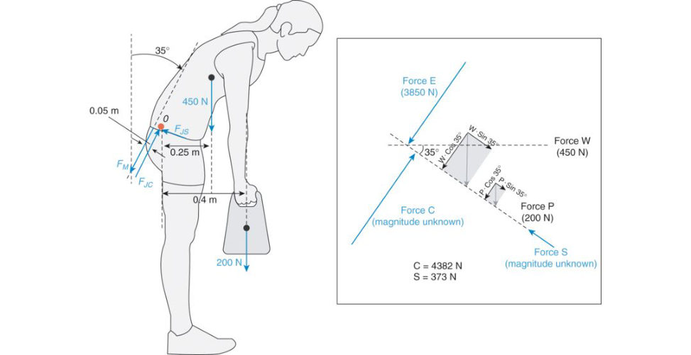
Assume the person weighs 70 kg and litis a 20 kg weight. The spine is flexed approximately 35°. The three principle forces acting on the lumbar spine a t the lumbar sacral level are: 1. Force produced by the weight of the upper body, W. 2. Force produced by the weight of the object, P. 3. Force produced by the contracture of erector spinae muscles, E. Because these three forces act at a distance from the centre of motion of the spine, the y create moments in the lumbar spine. Two forward-bending moments and a counterbalancing moment of the erector spinae muscle. For the body to be in moment equilibrium the sum of the moments acting on the lumbar spine must be zero. Clockwise and counterclockwise must balance. ∑ M = 0 W × 0.25 m + 200 N × 0.4 – FM × 0.05 = 0 450 N × 0.25 m + 200 N × 0.4 – E × 0.05 m = 0 E × 0.05 m = 112.5 Nm + 80 Nm E = 3850 N
Calculate the compressive force exerted on the disc.
C is the sum of the compressive forces acting over the disc which is inclined 35° to the transverse plane. The compressive force produced by the weight of the upper body W which acts on the disc inclined 35°. W × cos 35°
The force produced by the weight of the object P which acts on the inclined disc at 35°.
P × cos 35°
The force produced by the erector spinae muscles, which acts approximately at a right angle to the disc inclination.
The magnitude of C can be found through the equilibrium of forces:
∑ F = 0
W × cos 35° + P × cos 35° + E – C = 0
450 N × cos 35° + 200 N × cos 35° = 3850 N – C
C = 368.5 + 163.8 N = 3850 N
C = 4382 N
The shear component for the reaction force on the discS) is found in the same way.
450 N × sin 35° + 200 × sin 35° – S
S = 373 N
Figure 26.11a FBD of spine.
Practise drawing out a FBD of the spine as it is definitely known to be asked in a viva and trying to drawout for the first time in the exam from first principles is generally going to be doomed to failure (Figure 26.11a). The other viva scenario is the influence of litiing technique on spinal forces. An increase in the distance between the object being lifted and the spine increases the forward bending moment. Reaching too far for an object will induce substantially higher spinal loading (Figure 26.11)
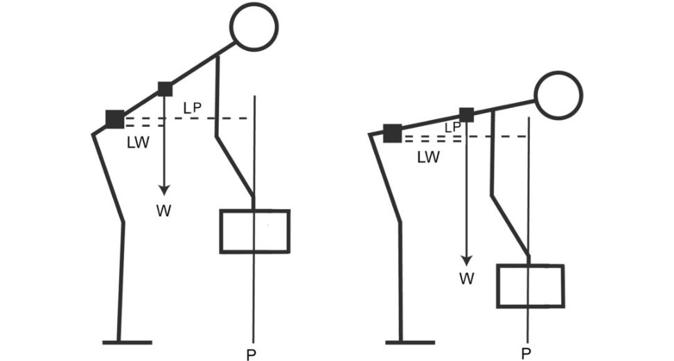
Figure 26.11b Candidate’s diagram FBD spine. Influence of litiing technique on spinal forces.The upper bodyweight and force exerted by the weight act in front of the disc and create forward bending moments. LW:lever arm for bodyweight, LP-lever arm for weight carried in hand.
Notes
1. To try and catch a candidate out, to be clever or just because it is something that should beknown and tested.
2. In the real exam the testis not about teaching. It is about how much a candidate knows. As such, the examiners will move past a point if a candidate doesn’t know it.
3. These terms are often incorrectly interchanged in various internet PPP. Yield strength is often described as the point at which elastic behaviour changes to plastic behaviour.
4. A different route whereby to get to the same destination.
5. As such this viva question can be asked across so many different Section 2 basic science viva topics.
6. Blu Tack is a reusable, putiy -like, pressure-sensitiv e adhesive produced by Bostik, commonly used to attach lightweight objects to walls, doors or other dry surfaces.
7. Practise beforehand being able to trot out these general assumptions while a t the same time being able to draw the asked for FBD.